Medical Assignment: Machine Learning-Based Diabetes Management

Question

Task:
Your medical assignment task is to prepare a dissertation on the topic “Early-stage diabetes and hospitalized diabetes patient readmission prediction with machine learning”.

Answer

Abstract
The concept of machine learning evolved in the present context of medical assignment has the potential to improve health systems by analyzing clinical data of millions are able to create forecasting models, screening and diagnostics. This machine learning systems leverage human intelligence or vast volumes of data to make a clinical decision. Machine learning can study large volumes of historical data and discover new knowledge that can forecast the potential trajectory of a person's wellbeing. Machine learning is important for delivering customized healthcare that integrates a wide range of personal data.Purpose of the study is to create models to predict early-stage diabetes in patients with machine learning models, and readmission of hospitalized diabetes patients using k means clustering model. The study emphasizes on two different cases of building machine learning models to predict early-stage risk and readmission of diabetes patients. The study uses two different datasets to analyze early-stage diabetes prediction and that of hospitalized patients’ readmission prediction by building machine learning models. The first dataset on early-stage diabetes prediction is used to create a predictive model for identifying the risk of diabetes. The second dataset on readmission of hospitalized diabetes patients in prediction of readmission to create a predictive model for identifying the risk of previously hospitalized diabetes patients. The study results area creation of relevant models to predict both the cases. For a given patient, it is predicted that they will be re-admitted within 30 days, and if they will not be provided with the patient's data, including the diagnosis and the medications they were taking.

Keywords: Machine learning, Healthcare, Predictive models, randomForest, k-means clustering, early-stage diabetes prediction, diabetes patient readmission

1. Introduction
Data mining is an increasingly important field of study in public health. By performing a variety of tasks, such as machine learning in research, data mining takes a wide variety of forms: applying a data-driven model to extract meaning from a set of data, mining of relevant variables of a data set, then evaluation of a model on these variables. The method of analysis of the study had implications beyond the mere potential effects of the procedure on the recipient's state of health. By comparing the risk of adverse events across surgical procedures for people of all ages, it was hypothesized that more procedures would have been performed before diagnosis and therefore in a different age group, which makes them less risky for unwanted results. Machine learning is booming and many research avenues are being explored to improve the technical performance of these systems, but also their suitability for targeted medical practices. Their cost must also be justified by a real added value for the doctor or the patient. The lines of research focus in particular on the processing of data, which is very heterogeneous, its structuring and anonymization, but also on the design of transparent systems for the user and well suited to the context of use.

1.1. Background
The number of patients in hospitals is growing rapidly, which means that it is becoming increasingly difficult to analyze, and even record, all patient data today. A good solution to this problem is machine learning, which facilitates the automation of data analysis and makes the healthcare system more robust. Machine learning applied to healthcare is the confluence of two fields: medical science and computer science. This alliance has enabled the medical field to make tremendous strides in healthcare.Diabetes is not only a dangerous disease but also one of the most common in the world. It is also a disease of entry, being itself one of the main causes of other diseases and leading its victims inexorably to death. Diabetes has the ability to damage various parts of the body, such as the heart, kidney, and nervous system. Machine learning is being studied as a way to detect diabetes markers early enough to save patients' lives. There are many algorithms that can be used to predict diabetes, such as Naïve Bayes, Decision Trees, Random Forests, and KNNs. The Naïve Bayes outperforms the rest when it comes to accuracy because of how good its performance is and how little computation time it takes.

The study emphasizes on using machine learning based diabetes management. Minimizing the impact of diabetes mellitus in the National Health System is one of the main challenges due to the high economic cost and the high rates of underdiagnoses and the variability of glycemic control in these patients. In addition, they tend to have a multi-pathological profile and an advanced age range. This makes it necessary to develop tools to improve the diagnosis of patients and better understand the resources they consume to improve clinical-care management.

1.2. Aims
The machine learning initiative will advance improved care and outcomes for people with diabetes, improving access to specialists and increasing the productivity of clinicians.

1.3. Research objective
The objectives of the research are;

• To use machine learning algorithms and build models for early-stage diabetes prediction, and;
• To use machine learning algorithms and build models for predicting readmission of previously hospitalized diabetes patients.

1.4. Research question
The research question formulated in the study is:

• Are machine learning models effective in predicting the early-stage diabetes?
• Do the machine learning models have higher accuracy in predicting the readmission of diabetes patients?

1.5. Hypotheses
Hypotheses of the study are;

• Effective application of machine learning models can predict early-stage diabetes
• Building predictive models can predict the diabetes patient’s readmission with high accuracy

1.6. Scope
Machine learning allows information to be analyzed in a similar way as if an experiment were carried out on a group of people. It gives an idea of how the results would have been if a specific intervention had been carried out. Although the study is a pilot, the novel combination of methods and data suggests that this type of study is valuable for evaluating programs and treatments in health systems and institutions. Digital health tools have the potential to improve research and treatment at a generally low cost, using routinely collected clinical and process data.The numerical approach can boast great performances in medicine, but it requires perfectly clean and well annotated data, such as those used for the recognition of melanomas. However, most of the medical data was not collected for the objective set by the software designer. They therefore pose many problems for their exploitation.

1.7. Rationale
Artificial intelligence (AI) is a quickly expanding field, and its contributions to diabetes, a global pandemic, have the potential to reshape the approach to the diagnosis and management of this chronic condition. Algorithms based on machine learning concepts have been developed to help predictive models of the probability of contracting diabetes or its related complications. Machine learning is playing an increasingly important role in many aspects of our lives, including healthcare. This can entail a variety of health-related activities such as the development of experimental medical treatments, the processing of patient records, and the prediction of disease care outcomes. However, the efficacy of machine learning approaches in forecasting the outcome of surgery and other medical methods is only partially known, at least in terms of predicting outcomes using data obtained by human physicians and other doctors. The significance of this study's research approach extends beyond the possible effect of the treatment on the recipient's medical condition. When the risk of adverse effects in the whole surgical process for patients of all ages is compared, it should be expected that further procedures will be done before diagnosis, because operations are performed in all age groups, minimizing the risk of adverse outcomes.

Machine learning is not a magical tool capable of transforming data into gold. Contrary to popular belief, it is a natural extension of standard statistical approaches. In today's healthcare systems, machine learning is a valuable and urgently important technology. With the vast volume of knowledge that physicians will use to analyze, such as the patient's personal genetic records, family disorders, gene sequences, prescriptions, social media habits, and hospitalizations at other hospitals, gathering observations to direct professional decision-making may be difficult. If algorithms gain more power, it is crucial to remember that these modern algorithmic decision-making methods cannot guarantee justice, fairness, or even accuracy. Regardless of whether the machine learning algorithm is high or poor, best methodological practices must be followed to ensure that the final outcomes are accurate and successful. This is particularly important in healthcare, where these algorithms have the ability to impact millions of patients' lives.

The oldest approach is based on the idea that we reason by applying logical rules (deduction, classification, hierarchy, etc.). The systems designed on this principle apply different methods, based on the development of interaction models between automata or autonomous software (multi-agent systems), syntactic and linguistic models (automatic language processing) or the development of ontologies. (knowledge representation). These models are then used by logical reasoning systems to produce new facts.The current systems, qualified as decision support, knowledge management or e-health, are more sophisticated. They benefit from better reasoning models as well as better techniques for describing medical knowledge, patients and medical acts. Algorithmic mechanics are basically the same, but description languages are more efficient and machines more powerful. They no longer seek to replace the doctor, but to support him in reasoning based on the medical knowledge of his specialty.

Machine learning is the science of building and programming a machine that can mimic human cognition. Some of the brightest scientists in the field of machine learning are in Canada, and our country has been at the forefront in this field for over 30 years. Machine learning presents immense possibilities for the transformation of human health. It is already helping to discover new drugs and make better medical diagnoses faster. It's not hard to imagine the near future where machine learning can reliably predict and stop diseases before symptoms appear. Theoretically, machine learning can, by examining a person's genome, recommend treatment options while limiting or eliminating side effects. Machine learning can streamline drug development to ensure researchers are looking at the most promising avenues and to help them find previously undiscovered pathways that could lead to new treatments and therapies. The emergence and growing use of machine learning and robotics will have a significant impact on healthcare systems around the world.

1.8. Importance
Artificial intelligence, machine learning, and machine learning have increased the profits of the medical industry. Although the contemporary world is on the verge of a new generation of technology and its potential is hardly understood, because of artificial intelligence and machine learning that the healthcare sector is seeing an increase in efficiency and revenue. Most large healthcare companies are currently investing in artificial intelligence to validate its position in current and future sectors.Traditional statistical models and machine learning are both machine learning methods. Traditional clinical research uses well-designed statistical models to analyze data from hundreds of patients, so it belongs to low-level machine learning in the field of machine learning.

With the reduction of human assumptions about algorithms, the status of machine algorithms in the field of machine learning has further improved. However, there has never been a specific threshold that can suddenly turn a statistical model into machine learning. Instead, both of these approaches exist on a scale defined by how many artificial hypotheses are imposed on the algorithm. Machine learning algorithms for image recognition, while requiring less human guidance, also require a vast volume of data to capture all of the sophistication, range, and detail found in real-world images. As a result, these algorithms often take hundreds of thousands of examples to obtain image features similar to the desired effects. A higher status in the field of machine learning does not mean an advantage, because different tasks require different levels of personnel participation. Although advanced algorithms are usually very flexible and can learn many tasks, they are often difficult to interpret. Algorithms in the low range of computer algorithms, on the other hand, typically generate output that is simple for humans to understand and perceive. Furthermore, the simplicity offered by the high end of the continuum necessitates the use of a vast amount of computational power to create and implement these algorithms.

High-end algorithms in the area of machine learning have been realistic and useful precisely because of the emergence of greater clinical data sources and faster machines over the last decade. Electronic clinical records (including laboratory scans, MRI scans, and diagnosis codes), activity trackers, genomic testing, and other websites may also include healthcare data. Big data is an opportunity, especially for healthcare applications. Machine learning is a technology that can incorporate and comprehend healthcare data on a massive scale. Machine learning allows online control of patient conditions and biomarkers that is both constant and unburdened. Furthermore, social media and online forums increase patient involvement in diabetes treatment. Technological advancements have aided in the optimization of diabetes resource use. These clever scientific reforms also resulted in improved glycemic regulation, with decreases in fasting and postprandial glucose levels, as well as glycosylated hemoglobin. Machine learning would usher in a paradigm shift in diabetes care, moving away from traditional management methods and toward the creation of precision data-driven care.

Machine learning (ML) is a rapidly expanding field of research with a great future. Its applications, which concern all human activities, make it possible in particular to improve the quality of care. ML is indeed at the heart of the medicine of the future, with assisted operations, remote patient monitoring, smart prostheses, personalized treatments thanks to the cross-checking of a growing number of data (bigdata), etc.The proponents of so-called strong machine learning aim to design a machine capable of reasoning like humans, with the supposed risk of generating a machine superior to humans and endowed with a consciousness of its own. This line of research is still being explored today, even though many ML researchers believe that achieving such a goal is impossible. On the other hand, proponents of so-called weak machine learning are implementing all available technologies to design machines capable of helping humans in their tasks. This field of research mobilizes many disciplines, from computer science to cognitive sciences through mathematics, without forgetting the specialized knowledge of the fields to which we wish to apply it. These systems, of very variable complexity, have in common that they are limited in their adaptability: they must be manually adapted to accomplish tasks other than those for which they were initially designed.

2. Literature Review
Diabetes is a condition that causes a slew of complications, including retinopathy, kidney disorders, hypertension, cardiovascular issues, and nervous system injury, among others, all of which can lead to death. Currently, it can be detected using one of three approaches that calculate blood sugar levels: a) a fasting blood glucose test; b) an oral glucose tolerance test; and c) a glycosylated hemoglobin measure, which reveals blood sugar activity over the previous months. The issue with such approaches is that they necessitate laboratory testing, which can take many days. In response to this problem, the present study proposes a predictive system to diagnose diabetes based on a Bayesian classifier (Hammoudeh et al, 2018). Bayesian networks are a probabilistic model through which it is feasible to construct a graph between the causes of an event - independent variables and its consequences - dependent variables. Bayesian classifiers allow classifying discrete and limited events - independent variables in a certain number of classes, defining a statistical function for each class. In defining these statistical functions, they take a training database as a reference. The method would be able to classify a new set of independent variables and decide which class they belong to depending on the statistical function that produces the highest value using these specified functions. In the case of diseases, the system operates from a series of simple parameters taken from the patient and does not require laboratory analysis (Mir, and Dhage, 2018, August).

CMS has developed a variety of initiatives to increase patient care outcomes as the healthcare system transitions toward value-based care. The Hospital Readmission Reduction Program (HRRP) is one of these services, and it limits payment of hospitals with higher-than-average readmission rates. One remedy for hospitals that are now being penalized by this scheme is to develop interventions that provide extra support to patients who are at a higher risk of readmission (Alloghani et al, 2019). A readmission to hospital happens after a patient discharged from the hospital is reinstated within a prescribed period of time. Readmission rates in hospitals with serious diseases have already been used as a patient quality barometer and as having a negative impact on healthcare costs. The Medicare and Medicaid Services Centers have thus established a reduction program for hospital admissions.It seeks to increase patient safety while simultaneously lowering healthcare costs by placing reimbursement penalties on hospitals with higher than planned readmission rates for specific conditions (Chopra et al, 2017, October). Despite the fact that diabetes is not currently included in the penalty measures, the initiative is constantly introducing more condition co-morbidities. While diabetes is not yet covered by penalties, more diseases are increasingly added to the list. Knowing what symptoms help to increase patient readmission rates and knowing which ones are admitted, saves hospitals millions of cash and improves the quality of care(Alloghani et al, 2019).

A high-priority health-care quality measure and cost-cutting target is hospital readmission. Diabetes is a major problem for hospitalized patients, on the other hand, is important, increasing, and expensive, with readmissions accounting for a significant portion of the cost. Diabetes mellitus is a prevalent comorbid disease among hospitalized patients due to its high prevalence (Dey et al, 2018, December). In recent years, federal departments and healthcare facilities have placed a greater emphasis on 30-day readmission rates in order to better understand the complexities of their patient populations and increase efficiency. The historical trends of diabetes treatment in patients with diabetes admitted to a US hospital were analyzed using a broad clinical database. A comprehensive clinical archive was analyzed to look at the past trends of diabetes treatment in diabetic patients admitted to a US hospital and to suggest potential directions that will result in a lower hospital readmission rate and better patient care (Chopra et al, 2017, October).

Readmissions to hospitals improve treatment rates and have a negative impact on the reputation of hospitals. The early-stage revision forecast helps patients at high risk of readmission to be given additional priority, thus maximizing the efficacy of the system and minimizing costs of health care. Machine learning can help provide more reliable forecasts than traditional methods. In this paper, a method for forecasting hospital readmission among diabetic patients is suggested that balances data engineering and neural networks' capacity to learn representations (Alloghani et al, 2019). When compared to other machine learning algorithms, convolutional neural networks and computer engineering were found to outperform them. A mixture of neural networks and computer engineering executed other machine learning algorithms when evaluated against real-world data (Chopra et al, 2017, October). Readmissions to hospitals improve health-care costs and damage hospitals' reputations. As a consequence, forecasting hospital readmissions in diabetics is a hot subject. Machine learning was introduced as an important method for predicting hospital readmissions among diabetic patients in this paper. When tested against real-world data, a blend of Convolutional neural networks and data engineering outperformed other machine learning algorithms (Alloghani et al, 2019).

Machine learning is essentially a multi-layer neural network (NN) that learns data representations at various levels of abstraction. Unlike standard machine-learning methods, which have a restricted potential to progress when exposed to more data, machine learning can scale efficiently even with raw data. Two types of neural network architectures are investigated: standard artificial neural networks (ANNs) and convolutional nets (CNNs). Since CNNs outperformed ANNs for the same layers, only the CNN findings are presented (Dey et al, 2018, December). Classifiers based on neural networks can distinguish between non-linearly separable groups and generalize far. Classifiers based on neural networks may discern non-linearly separable groups and generalize well beyond the examples shown. Furthermore, deep layers remove a significant amount of feature engineering work that was previously needed for shallow classifiers; deep neural networks will automatically learn the representation. Increasing the number of layers in a neural network increases the representation's selectivity and invariance, allowing a classifier to draw highly complex functions of its inputs that are sensitive to small differences that differentiate one class from another while being indifferent to vast irrelevant differences between instances of the same class (Hammoudeh et al, 2018).

According to the report, diabetic patients have a higher chance of readmission than non-diabetic patients. It employs logistic regression to classify inpatient stays, race, diabetes prior to stay, and heart problem as good predictors, but it does not take into account the problem of class imbalance. Inpatient and outpatient appointments, primary diagnosis, manner of admission, and patient status were all central variables in their study, which used a support vector machine (Joshi, and Alehegn, 2017). Another research showed that decision trees outperformed logistic regression and nave Bayes in forecasting diabetic patients' readmission. The readmission department, the duration of stay, and the patient's age are all contributing factors (Hammoudeh et al, 2018). Readmission department, duration of stay, and patient medical background are all mitigating factors, but they haven't discussed the problem of class imbalance. However, as compared to nave Bayes and decision trees, logistic regression produces better outcomes. Another research contrasts Bayes, random forest, adaboost, and neural networks to show that random forest increases prediction performance. The number of inpatient stays, discharge disposition ID, admission source, and number of diagnoses were all found to be good predictors, but they did not solve the issue of class imbalance (Dagliati et al, 2018).

Although previous study has shown the usefulness of machine learning in forecasting hospital readmission for diabetic patients, none of the studies took into account the data set's intrinsic class imbalance. Furthermore, the accuracy of the methods and the resulting collection of related features are highly variable. It aims to account for the issue of class imbalance in a more recent review, showing that logistic regression outperforms random forest and SVM. Sex, age, time of diagnosis, BMI, and HbA1c are all important factors in type-2 diabetes (Alloghani et al, 2019).

Previous experiments, according to the literature, have shown inconsistent findings and have failed to resolve the issue of class imbalance. Although the study sought to address this problem, it was confined to patients with type 2 diabetes and had a much-reduced data collection. This thesis explores the issue of class disparity by using a much broader sample collection that covers patients with various forms of diabetes. In addition, the report aims at a wider variety of machine learning methods, including those that haven't been explored before (Mir, and Dhage, 2018, August). The research employs a variety of pre-processing methods, as well as function analysis and model output analysis. Diabetes Mellitus (DM) is a progressive condition characterized by the failure of the body to metabolize glucose. Early diagnosis decreases the cost of care and reduces the risk of more severe health problems for patients. Machine learning has multiple purposes in healthcare and can be used wherever data is generated and utilized, such as in clinical trials, diagnosis and even in managing chronic conditions such as diabetes. In theory, machine learning brings automation, personalization and simplicity to aspects of healthcare (Joshi, and Alehegn, 2017).

Predictive analysis through machine learning can help people with diabetes to identify whether they have higher risk for developing comorbidities and complications, such as cardiovascular disease or neuropathy, before they emerge or progress. For example, companies have previously investigated how machine learning could be used to automate screenings for diabetic retinopathy, which is recognized to be one of the leading causes of blindness in working-age adults (Kumar, and Pranavi, 2017, December). Using data in this way will help us connect the dots between various conditions and healthcare settings, creating a more holistic healthcare ecosystem than we have today. This is particularly an important touch point for people with diabetes to facilitate care more virtually with telehealth and healthcare portals serving as key opportunities to transfer data for remote patient monitoring and electronic medical records (Saru, and Subashree, 2019).

Random woodlands are a decision grade raising the technical variation in that they allow random growth branches within the selected subspace which differentiates from other grades. The random forest model uses a number of random base regression trees to forecast the result. At each random base regression, the algorithm selects a node and divides it to grow the other branches. Since Random Forest blends multiple trees, it is important to remember that it is an ensemble algorithm. Ensemble algorithms, in principle, incorporate one or more classifiers of multiple types (Joshi, and Alehegn, 2017). The Random Forest approach is used as an approach to optimize decision-making. The algorithm selects the sub-set, which is considerably smaller than all features in the process, and is based on the best sub-set function. Since databases of large-scale subsets appear to raise computing sophistication, a limited subset size decreases the responsibility of deciding on the number of features to break. As a result, narrowing the attributes to be learned increases the algorithm's learning speed (Mir, and Dhage, 2018, August).

The methods used to treat illnesses have a significant impact on the patient's treatment outcome, including the likelihood of re-admission. An increasing number of publications indicate that there is a pressing need to investigate and classify the contributing factors that play crucial roles in human diseases. This may aid in the discovery of the pathways that underpin disease progression. In a perfect future, this can be obtained by experimental findings that demonstrate useful approaches that outperform other experiments (Saru, and Subashree, 2019). Many techniques were built in the same way to accomplish certain goals by using novel statistical methods on large-scale datasets. As a result of this observation, the requisition has been given. This result requires proper patient treatment practices, in particular for those admitted to the intensive care ward. However, Non-ICU patients do not have the same recommendations completely available. It results in inadequate inpatient management procedures such as the number of medications, lab tests performed, discharge, minor modifications or adjustments at the time of discharge, and elevated re-admission rates (Joshi, and Alehegn, 2017).

Nonetheless, such a point has not been confirmed, nor has the impact of these causes on diabetes re-admission. The study hypothesis has also come that the duration of the hospitalization, the number of laboratory examinations, number of medications, and the number of diagnoses is related to re-admission rates. However, the study noted improvements as partial control considerations that can moderate the admission. Any re-admissions can be avoided, although this includes evidence-based interventions (Kumar, and Pranavi, 2017, December). In a retrospective cohort analysis, researchers looked at simple diagnosis and 30-day re-admission rates for patients at Academic Tertiary Medical Centers and found that re-admissions can be prevented within 30 days. According to the study, re-entries within 30 days can be avoided technically. As a subtext of the conclusion, the authors believed that these re-admissions events were linked to symptoms identical to the primary diagnosis directly or indirectly. Studies show a greater likelihood of reacceptance for acute heart failure in patients hospitalized for heart failure and other related disorders. The care given, the reported health result at discharge, and other pre-existing health problems all play a role in the recurrence of the cardiac disease (Shankar, and Manikandan, 2019).

Machine learning will lead to significant benefits for both patients and providers as technology advances. Patients will benefit from methods that evaluate other physiologic factors as well as automatic insulin distribution. Diabetes experts would have better statistics and new diabetes treatment concepts at their disposal. To remain experts in diabetes technologies, they will need to keep up with new offerings. The potential of comparable techniques to extract patterns and construct models from data underpins the strength and usefulness of these approaches (Saru, and Subashree, 2019). The above fact is particularly relevant in the Big Data period, particularly when terabytes or petabytes are included in the data collection. The foregoing fact is especially relevant in the big data era, where datasets can be terabytes or petabytes in scale. As a consequence, the availability of data has greatly helped data-driven biology science. One of the most significant scientific applications of such a hybrid area is prediction and diagnoses for conditions that endanger individuals and/or decrease the quality of life, such as diabetes mellitus (DM) (Mir, and Dhage, 2018, August).

Diabetes is becoming more popular in people's daily lives as their living standards increase. As a result, learning how to detect and evaluate diabetes easily and reliably is a subject worth exploring. The use of fasting blood glucose, immunity to glucose and random blood glucose levels in medicine is diagnosed with diabetes. The quicker we get a diagnosis, the better it would be to monitor. Machine learning can assist people in making a provisional diagnosis of diabetes mellitus based on their regular physical assessment results, and it can even be used by doctors as a guideline. The most critical challenges with machine learning approaches are how to pick relevant features and the proper classifier (Kumar, and Pranavi, 2017, December). The model is high and acceptable for the prediction of patients with diabetes with specific widely used laboratory findings. These models will be combined with the online computer program to support physicians in the prediction of patients who experience diabetes in the future. This model was developed and validated by a Canadian population to be more specific and powerful than existing models for American or other populations (Joshi, and Alehegn, 2017).

Many diabetes prediction algorithms have been used lately, including conventional approaches to machine learning, such as vector support (SVM), decision tree (DT), logistical regression and more. The key feature study of diabetes and the neuro-fuzzy inference is used to distinguish diabetes from healthy people. The scientists proposed the LDA MWSVM process, which uses the QPSO algorithm and the weighted lesser squares vector machine to predict type 2 diabetes. The researchers have identified LDA-MWSVM (Joshi, and Alehegn, 2017). The authors used Linear Discriminant Analysis to minimize dimensions and derive features from this approach (LDA). The approach has been developed to work with massive data sets (Dey et al, 2018, December). Predictive models based on logistic regression have been designed to address high-dimensional datasets for various onsets of the form 2 forecast. Support Vector regression (SVR), a multivariate regressive problem with a focus on glucose has served to model diabetes. Furthermore, a growing number of studies have suggested a new ensemble technique, rotation forest, which incorporates 30 machine learning approaches to increase accuracy (Dagliati et al, 2018).

The data-intensive essence of diabetes diagnosis and treatment lends itself to the incorporation of machine learning for performance improvement and the discovery of new approaches. The researchers used numerous types of machine learning algorithms in their key evaluations of master learning techniques used in various DM studies. Different studies on several smart DM assistants developed using techniques of artificial intelligence have also been published (Shankar, and Manikandan, 2019). This section aims to cover the algorithms of machine learning used in primary study and the numerous intelligent helpers in DM tech (Dey et al, 2018, December). Prediction models based on logistic regression were developed to resolve high-size datasets for multiple start-ups in the type 2 diabetes prediction. Support Vector regression (SVM) has been used to predict diabetes that is a glucose-focused multivariate challenge. Furthermore, a growing number of studies have suggested a new ensemble technique, rotation forest, which incorporates 30 machine learning approaches to increase accuracy (Faruque, and Sarker, 2019, February).

3. Empirical based projects
3.1. Methodology
The methodology selected is analysis using two datasets that will be analyzed using Python. Also, the specific method used includes the machine learning classification algorithm like Logistic Regression; Decision Tree; Binary Classification, etc. The analysis using the methodology combines both the datasets strategically using machine learning and data analysis for diabetes management. The strengths of the selected methodologiesare that these machine learning models has a higher speed when training and querying large numbers. Even if a very large-scale training set is used, there are usually only a relatively small number of features for each item.The training and classification of items are only mathematical operations of feature probabilities. Most of these methods are not very sensitive to missing data, and the algorithm is relatively simple, often used for text classification.Moreover, they are easy to understand while interpreting the results. The limitations of the models in the selected machine learning methodology are that they are very sensitive to the expression form of the input data. Since the assumption of the independence of sample attributes is used, the effect is not good if the sample attributes are related.

3.2. Early-Stage Diabetes
The survey on the diabetes management with machine learning depicts that machine learning and the individuals who may have diabetes will be identified. Material was contained on medical exams, blood and urine samples, and questionnaires for patients. Diabetes has a higher risk of major health complications, including heart failure and cancer, and is thus important for avoiding it to decrease the risk of disease and premature death. Machine learning could allow high-risk groups of potential patients with diabetes to be better identified than using current levels of risk. Furthermore, it may be possible to raise the number of visits to health workers to avoid eventual diabetes onset (Sowah et al, 2020).

Computers learn without express programming in machine learning. A machine learning formula increasingly increases pattern detection with any introduction to new data. Machine learning allows information to be analyzed in a similar way as if an experiment were carried out on a group of people, giving an idea of how the results would have been if a specific intervention had been carried out (Donsa et al, 2015). Machine learning is a fast-expanding area that will change the method for the diagnosis and management of this chronic condition by applying itself to diabetes as a global pandemic. The principles of machine learning were used to build algorithms to support predictive models of the chance of developing diabetes or associated complications. Digital therapy has become a well-known lifestyle treatment procedure for management of diabetes(Singla et al, 2019). Patients are becoming more self-managed, and the assistance of therapeutic decision-making is available to both them and health care practitioners. Machine learning helps patient signs and bio-markers to persist, unburdened, remotely controlled. Social networking and online forums also increase patient commitment to the treatment of diabetes. Development in technologies helped to optimize the use of diabetes tools. These smart technological reforms together have led to an improved glycemic regulation, a decrease in fast glucose and glycosylated hemoglobin levels. Machine learning introduces a change in diabetes treatment model from traditional management techniques to data-driven care growth (Sharma, and Singh, 2018, July).

The difficulty with medications is that various types of drugs are possible to cure the illness. If the diabetic population grows, new therapies are continuously developing. In certain cases, diabetics should take other medicines in order to combat chronic diseases such as elevated cholesterol and high blood pressure. With the age of the patient and other physical conditions, the efficacy of treatment varies (Kaggle. 2021). Depending on the condition of the client, there are often many side effects, and treatment can be costly. Every three months the efficacy of treatments is assessed by a blood test called machine learning.Machine learning introduces a change in diabetes treatment model from traditional management techniques to data-driven care growth (Sowah et al, 2020).

The average blood glucose level in the last three months is measured by machine learning. To date, drug prescription has traditionally been a test-and-error strategy and more than half of the patients with diabetes have failed to reach the World Diabetes Journal. It is also unpredictable for patients to choose and treat the most appropriate drug or drug combination which is safe, cheaper, and more tolerated (Donsa et al, 2015). A collaborative policy support mechanism to make it easier to make pharmaceutical decisions on type 2 diabetes possible for physicians and patients. Machine learning approaches are used to forecast the risk of specific outcomes from a single medication regime by integrates electronic health data for tailored advice. In order to grasp easily doctors and patients, the systems measure drug regimens side to side, estimating the effectiveness, probability of effects and cost (Singla et al, 2019).

The trouble with medicines is that various drug formulations can cure the condition in several ways. As the diabetic population grows, new medications are increasingly emerging. In order to treat common diseases such as elevated cholesterol and high blood pressure, diabetics also continue to take other drugs. With the patient's age and other physical conditions, the potency of these medicines varies (Sharma, and Singh, 2018, July). In this method, the effectiveness, risks of side effects and costs are measured side by side, and are readily grasped by doctors and patients. The most prevalent form of Type 2 diabetes effects more people as people grow up. This disease has also escalated dramatically due to the spread of western diets and lifestyles to developing countries. Diabetes is an incurable metabolic illness that happens when high blood sugar is present, and may have deadly effects. Today, medicine, nutritious diets and exercise will regulate diabetes. It is also unpredictable to choose and administer the most appropriate mixture of prescription, which is stable, cheap and well tolerated by patients as well (Plis et al, 2014, June).The scientists funded by NIH use promising technologies to help people monitor diabetes more effectively. Systems of artificial pancreas regulate blood glucose levels and automatically provide insulin or an insulin mixture with another essential hormone. Devices can be configured and used easily. To launch, the unit just needs to reach the body weight. The machine lifts the blood glucose level heavily and frees the patient and makes it possible for them to live less and more spontaneously. More participants and over prolonged periods of time try many different devices. The researchers evaluate the protection, user-friendliness, participants' physical and emotional wellbeing and device costs (Neborachko et al, 2019).

If a patient has type 1 diabetes, the blood glucose levels can be erratic and potentially risky. In an incredibly demanding situation, the artificial pancreas worked very well. Eventually, people with diabetes will have the freedom they have avoided in the past to engage in a healthy manner. For people with diabetes, an artificial pancreas approved by the FDA is already available. Diabetes systems will be completely automated for the public in the coming years. Researchers are considering how those devices are used in people with type 2, pregnancy, and other disorders including high blood glucose levels (Marling et al, 2012).These technologies help to monitor diabetes and improve the health of people who use it. Although there will be tools to make managing the diabetes simpler in the future, the patient will learn how to handle the diabetes using today's tools for a long and stable life. Medicines, glucose sensors and insulin pumps are available now to support patients suffering from diabetes (Plis et al, 2014, June).

The data is structured so that each row represents a patient and the columns each property or attribute that is used for learning of the expert system. Another design aspect of the expert system consists of the use of solutions based on machine learning with a supervised approach, due to the nature of the data sets where the Finds important historical information for the training of the expert system, which generates decision trees (Donsa et al, 2015). The variables previous medications, observations of the doctor and date of diagnosis, because they do not intervene directly acritical measures to determine whether or not a person may have the disease. As a concrete example, the date of diagnosis: anyone can come any day for a study diabetes and can be positive or negative. In the case of the attribute of number of pregnancies, patients had zero pregnancies, which does not necessarily mean that it is male or female, but, unlike from the date of diagnosis, this data in combination with the others, is outstanding for predicting disease, regardless of sex of person (Neborachko et al, 2019).

With the diabetes data set, a pre-processing of the information to determine if a person can positively suffer from the disease. It is important to emphasize that the glucose measurement stands out importantly with the rest of the variables as a measure of suffering from positively the disease, however, as mentioned in stage 2 of the methodology is not always reliable (Islam, and Jahan, 2017). Using the machine learning tools, decision trees were generated, consisting of a type of predictive model where a graph with tree structure for data classification. Each node of the tree symbolizes question and each branch corresponds to a specific answer to that question, that is, a predicate. The confusion matrix resulted with 93 cases of false positives and 108 cases of false negatives. This is because there are register values such as the number of pregnancies, which in some cases is zero. Therefore, these of the application favors to an acceptable extent the prognosis of diabetes, However, if any information is lacking, it is considered not to be prone to disease (Marling et al, 2012).

By applying an adequate methodology for the design and development of systems experts can achieve objectives satisfactorily, as in the case of the Weiss and Kuligowski methodology. On the other hand, machine learning has several knowledge machine algorithms, which can be useful to be applied on various data sets through the different interfaces that offers, as the option of Explorer and Datasets, which were worked in this case of study, or to be included in other applications. Furthermore, both tools, contain what is necessary to conduct data transformations, grouping, regression, clustering, correlation and visualization tasks (Kaur, and Kumari, 2020). Because they are designed as extensibility-oriented tools which allows to add new functionalities to a project, because it can be combined with other programming languages such as Prolog, for generation more robust expert systems (Khan et al, 2017, December).

3.3. Readmitted diabetes patients
Machine learning techniques allow to automatically identify patterns and even make predictions based on a large amount of data that could be extracted from the computer systems used to ascertain information on readmission of diabetes patients. The analysis Clustering or grouping is a technique that allows exploring a setoff objects to determine if there are groups that can be significantly represented by certain characteristics, in this way, objects of the same group are very similar to each other and different from objects in other groups (Hosseini et al, 2020).

The results obtained by comparing the relevance of different attributes as well as the use of two of the most popular algorithms in the world of machine learning are presented: neural networks and decision trees. Automatic classification of blood glucose measurements will allow specialists to prescribe a more accurate treatment based on the information obtained directly from the patients' glucometer (Hosseini et al, 2020). Thus, it contributes to the development of automatic decision support systems for gestational diabetes. This high level of glucose in the blood is transferred to the fetus causing various disorders: excessive growth of adipose tissues, which increases the need for caesarean section, neonatal hypoglycemia and increased risk of intrauterine fetal death (Dagliati et al, 2018). It also increases the risk of type 2 diabetes once the gestation period is over for both the mother and the fetus. The project proposes the development of intelligent and educational tools for the survey based on neurodiffuse techniques integrated into a telemedicine system. Telemedicine systems have been used with success on numerous occasions in diabetes and the integration of decision support tools in this type of system helps a better interpretation of the data (Abhari et al, 2019).

In the survey, glycemia is regulated through diet, physical exercise and, on some occasions, insulin administration is required. To do this, patients must control their blood glucose levels with the help of a glucometer, taking at least 4 measurements a day, one on an empty stomach and the other three after each main intake. These data, glucose level and associated intake, they are recorded by the patients in a control book that they teach the specialist weekly (Bastani, 2014). The specialist uses this information to guide the corresponding diet and the administration of insulin if necessary. Most glucometers allow patient measurements to be stored, thus avoiding the tedious task of writing down the values in the control book. This has a great advantage over the possible absence and unreliability of the data recorded manually, and opens the possibility of processing the data automatically and integrating them into telemedicine systems and helps with decision-making (Khan et al, 2017, December).

Nevertheless, the information obtained from the glucometer is insufficient to be examined directly by a specialist, since it is essential for them to know the intake to which each measurement is associated and whether it is preprandial or postprandial data. Given the data stored in the memory file of the glucometer, the specialist is forced to decipher which intake corresponds to each measurement. Therefore, the list of values provided by the glucometer must be classified according to the intakes so that the specialist can determine the corresponding treatment (Bastani, 2014). The machine learning program learns from experience if it improves its performance in carrying out a specific task by increasing that experience. Machine learning algorithms make it possible to design programs capable of learning from past data. In the case, it will allow us to design a classifier capable of learning from previously classified patient data, in order to classify new data (Abhari et al, 2019).

4. Findings, Conclusions, Reflection, Recommendations
4.1. Findings
4.1.1. Early-Stage Diabetes Prediction

Reading the data
Seeing the first 5 rows of the dataset

Table 4.1.1.1. showingfirst five rows of dataset

Getting the statistical parameter values for each column

Table 4.1.1.2. showingstatistical parameter values for each column

Exploratory Data Analysis
Distribution of target variable

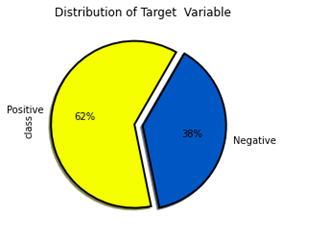
Figure4.1.1.1. showingdistribution of target variable

Distribution of target variable versus gender

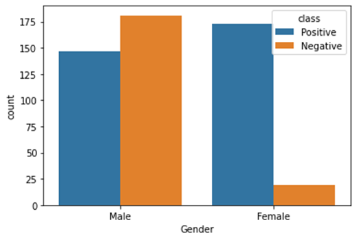
Figure4.1.1.2. showingdistribution of target variable versus gender

Distribution of target variable versus other features

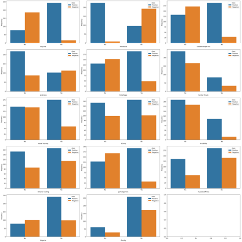
Figure4.1.1.3. showingdistribution of target variable versus other features

Seeing how features are correlated to the target variables

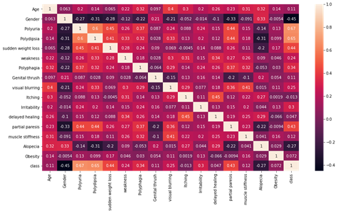
Figure4.1.1.4. showinghow features are correlated to the target variables

Feature Selection

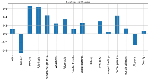
Figure4.1.1.5. showingfeature Selection

Machine Learning Models
Logistic Regression

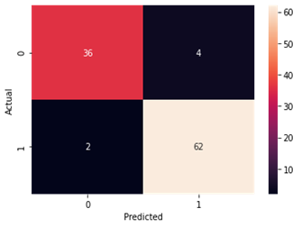
Figure4.1.1.6. showinglogistic regressionconfusion matrix

Support Vector Machine
Accuracy and Confusion Matrix

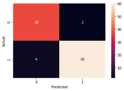
Figure4.1.1.7. showingsupport vector machine confusion matrix

K-nearest Neighbour
Accuracy and Confusion Matrix

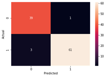
Figure4.1.1.8. showingK-nearest Neighbour confusion matrix

Naive Bayes
Accuracy and Confusion Matrix

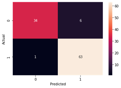
Figure4.1.1.9. showingNaïve Bayes confusion matrix

Decision Tree Classifier
Accuracy and Confusion Matrix

Figure4.1.1.10. showingdecision tree classifier confusion matrix

Random Forest Classifier
Accuracy and Confusion Matrix

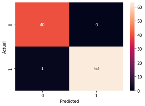
Figure4.1.1.11. showingrandom forest classifier confusion matrix

4.2. Hospitalized diabetes patient’s readmission prediction – k means clustering
4.2.1. Code

Reading the data
Seeing the first 5 rows of the dataset

Table 4.2.1.1. showingfirst 5 rows of the dataset

Getting the statistical parameter values for each column

Table 4.2.1.2. showingstatistical parameter values for each column

Plotting the bar graph to get the frequency of each categories present

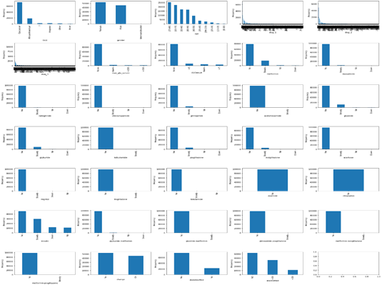
Figure4.2.1.1. showing bar graph to get the frequency of each categories present

Check for readmitted patients and remove all visits other than the 1st visit

Table 4.2.1.3. check for readmitted patients and visits other than the 1st removed

Clustering Algorithm

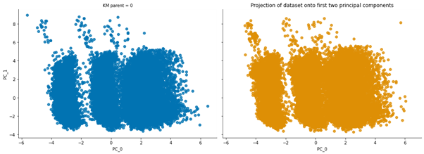
Figure4.2.1.2. showing clustering algorithm

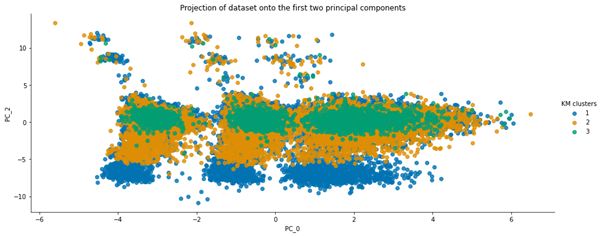
Figure4.2.1.3. showing projection of dataset onto the first two principal components

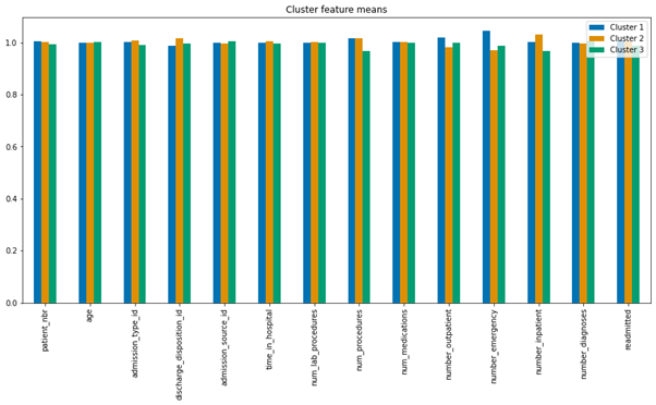
Figure4.2.1.4. showing cluster feature containing the means of each feature

Table 4.2.1.4. showing scaling of the means to better represent cluster differences

5. Conclusion
5.1. Early-stage diabetes prediction
Diabetes is the fastest growing chronic life-threatening disease, affecting over 422 million people worldwide. Type 2 diabetes is caused mainly by environmental factors and lifestyle. It is a slowly developing disease in which metabolic rates begin to develop long before they develop into illness, and is usually diagnosed with a fasting sugar test. The dataset used here contains reports of diabetes symptoms from 520 patients. It includes data about people, such as their age, gender, and the symptoms that diabetes can cause. The dataset was generated from a direct questionnaire and completed under the supervision of a physician from Sylhet Diabetes Hospital in Sylhet, Bangladesh. This dataset looked at other metabolic indicators for diagnosing people with prediabetes.

From analyzing the dataset, the number of rows and columns in the dataset were evaluated. There were 520 rows (patient) in the dataset. There were 17 columns (features) in the dataset. From getting the statistical parameter values for each column, out of the 17 features, only one feature is integer.All other 16 features were non-numeric.There were no null values present inside the dataset. So, no need of data cleaning.Analyzing the number of positive and negative class in the dataset, it was ascertained that there were 320 subjects with positive class and that there were 200 subjects with negative class.

Exploratory Data Analysiswas performed with the dataset. Distribution of target variable depicted that there were 62% patients from positive class.There were 38% patients from negative class.From analyzing the distribution of target variable versus gender, it was ascertained that there were less subjects of female for negative class.For male, the positive and negative class were not much different.Number of females for positive class is comparable to male positive and negative class.There were no missing values in the dataset. The data form of this dataset has 16 attributes that was used to predict outcomes: a positive class variable which indicates that the person has diabetes, and the class variable is negative which indicates that the person does not have diabetes. Predicting diabetic class all attributes except age have categorical data with two unique outcomes Patient ages ranged from 16 to 90. There are no missing values in the dataset.61.5% of patients were diabetic and 38.5% were non-diabetic. 37% and 67% of patients were women and men, respectively. 90% and 45% of women and men suffered from diabetes, respectively.

Polyuria and polydipsia had the highest correlation (correlation coefficients of 0.67 and 0.65, respectively) with diabetes. Age had a low correlation (correlation coefficient 0.11) with diabetes. Age was categorized (1.15–25, 2, 26–35, 3.36–45, 4.46–55.5.56–65, 6. and above 65) to further explore its association with diabetes. In the age distribution of patients, there were more people in age group 4 (46–55 years). There is no statistically significant association between age group and diabetes, as diabetes is equally distributed across all age groups. The chi-square test was performed, which gave a p-value of 0.076. A p-value> 0.05, so we cannot reject the null hypothesis that there is no association between age group and diabetes. After the chi-square test was performed to investigate the relationship between polyuria and diabetes, the resulting p-value was less than 0.05. So we reject the null hypothesis and conclude that there is a significant link between polyuria and diabetes.

The distribution of target variable versus other features was performed using visualization i.e.,countplot. From the above countplot, following conclusion can be made.If there is polyurea then there were higher chances of getting positive.If there is polydepsia then there were higher chances of getting positive.Similar conclusion can be made with other plots as well.Data Preprocessing was done and it was analyzed how features were correlated to the target variables. From heatmap it is clear polyurea and polydipsia were highest correlated with target value.Obesity and itching were least correlated with the target values.

From creating the machine learning models, the dataset was analyzed. The accuracy of the Logistic regression machine learning model is 96.15%. The accuracy of the Support vector machine learning model is 94.23%. The accuracy of the K-nearest neighbor model is 96.15 %. The accuracy of the Naive Bayes model is 93.26 %. The accuracy of the Decision Tree Classifier model is 99.04 %. The accuracy of the Random Forest Classifier model is 99.03 %. Exploratory data analysis was performed on the dataset. Feature selection was done to get the optimal features. Five different machine learning algorithms was implemented. Random Forest and Decision Tree model gives the best results. These are good forecast indicators. Both common and less common symptoms of diabetes can be used to predict diabetes early using a machine learning approach. The MLP machine learning model is well suited due to its accuracy.

5.2. Hospitalized diabetes patient’s readmission prediction with k means clustering
From assessing the dataset, number of rows and columns in the dataset were ascertained. In the dataset, there are 33,243 rows (number of subjects).There are 50 columns (features).The statistical parameter values for each column were obtained. There are only 13 columns out of the 50 columns.This means that in rest of the columns there are non-numeric values.These non-numeric columns cannot be given to the ML model. So,they are analyzed and converted into appropriate form.

After cleansing the data, the weight has almost 96.47% missing values. Payer code has around 84.43 % missing values. Medical Specialty has around 36.60 % of missing values. Also race has 2 % of missing values. diag_1, diag_2, diag_3 has very few missing values. So, these columnsare dropped form analysis. Since we are solving the readmission problem, if patient dies there is no point of readmission. So, those data points are also removed.

From the bar graph, it is evident that citoglipton and examide have only one application.Also, for gender features there are some unknown values with missing data. The categorical variables were transformed into binary form. The figures included varying numbers of hospitalizations, emergency department visits and ambulatory visits with a given patient in the last year. There are (rough) estimates of how much an individual has used in the last year's hospital/clinical care. These three have been introduced to construct a new variable called the use of operation.

From analysing the number of medication changes taken by the patient, there are total 23 medication taken. Out of which 2 medication is never used.Medication changes may have correlation with lower admission rate. The number of medications changed was analyzed and it was used in understanding the severity of the condition.

K-means clustering analysis was performedand the following conclusions were made. Patients in the first cluster spent between a third and half a day longer in hospital. Patients in the first cluster had about 5% more lab procedures than those in clusters two or three, and were, on average, using between 15 and 25% more medicaments.Patients in the first cluster had a record of more encounters (inpatient, emergency, and outpatient).All clusters had circulatory diagnoses top. Patients on fewer/no diabetes medications were readmitted much more frequently for digestive problems, whereas patients with many were admitted more frequently for hormonal problems.

It can be difficult to know if a patient will be readmitted to hospital, this could mean that the patient did not receive the best treatment the last time they were hospitalized, or the patient could be misdiagnosed and treated for another medical condition. together. When a patient is first seen, it is not possible to predict whether he / she will be re-admitted or not, but laboratory reports and patient type details can be very helpful in predicting whether a patient can be re-admitted within 30 days. This dataset's key purpose is to assess whether a diabetes patient is readmitted in 30 days. It is expected in a given patient if they are re-admitted within 30 days, or whether patient records, including the diagnosis and drugs they were taking, are not presented.

The dataset covers ten years of health treatment in 130 US hospitals and advanced care networks (1999–2008). It has over 50 roles that present outcomes to patients and hospitals. Patient number, race, gender, age, method of hospitalization, time in hospital, medical specialty of the receiving physician, number of laboratory tests conducted, HbA1c test score, diagnosis, number of medications, diabetic drugs, number of outpatients, inpatients, and emergency visits one year before hospitalization, and so on are among the attributes contained in the results. The very first step in solving any data science case study is looking at and analyzing the data correctly. This helps you gain valuable insights and information. Statistical tools play a big role in visualizing data correctly. Machine learning engineers spend most of their time solving a problem by analyzing the data they have, and this step is considered an important step because it helps us understand the data accurately. The correct EDA gives interesting features to the data, which in turn influences our preprocessing and model selection criteria.

It is observed that the weight has the highest zero values - 96%. Medical specialty and payer code have zero values of 48% and 43%, respectively. The weight function can be omitted because the percentage of zero values is very high. The payer code and missing values in the medical specialty’s column can be found using imputation methods, as more than 50% of the data is available in both cases. The race column consists of Caucasian, African American, Hispanic, Asian, and other categories. It consists of 2.7% NaN values. The patients are predominantly Caucasian, followed by African Americans and least of all Asians. The nan values are filled with race mode. As expected, there are fewer patients less than 40 years old compared to patients over 40 years old. Most of the patients are in the 70–80 age group.

In Admission_type_id, most patients arrive with an emergency ID followed by a selective one. Some patients do not have admission type identifiers. There are also Null and Not mapped categories. The rank_disposition_id column is divided into 21 categories, which are then changed into 8 categories after careful observation. There are no patients who have died or are in hospice because we have already removed these lines from the data. On average, patients stay in the hospital for 4 days, while most patients stay for 3-4 days. Patients rarely stay longer than 12 days. It can be observed a positive bias in the plot. On average, 43 laboratory procedures are performed during an appointment with a patient. The peak is also found around 0–2 procedures, indicating that fewer laboratory tests have been performed in some patients.Most patients do not perform any tests other than laboratory tests. There is a positive bias.

The majority of patients do not visit the hospital. This is similar to the other attendance numbers seen. A new “visit” function is created that includes inpatient, outpatient and emergency visits, since all three are equally distributed. All three diagnostic functions contain codes that are classified into one of 9 groups. Groups are given in the research paper. These codes are divided into 9 categories and use them to diagnose diseases that fall under these 9 categories. In the second and third diagnoses, it can be observed that more patients are diagnosed with 4 - diabetes mellitus. Most patients are diagnosed with respiratory and other illnesses. The nan category also increases with the diagnosis number. It is represented in the function as -1.There are 23 remedies in total, and values are given for each remedy. The analysis revealed that 3 drugs were not prescribed to any patient. These 3 functions do not help to determine if the patient has been readmitted to hospital within 30 days, as all values are the same. Thus, these features have been removed from the dataset. Medicines can be combined into one function, and the number of medicines that patients have been taking can be calculated. Custom drug coding was done with any dosage change resulting in 2, consistently given as 1, and if no drug is required, it is presented as 0.

More than 50% of patients did not change their medications, the rest changed their medications. The sign of change has been coded: 0 means no change and 1 means drug change. Most of the patients were prescribed diabetes medications. For DiabetesMed, a 0 was coded for unprescribed and 1 for a prescription. This is a variable that we must predict. This is the number of days until hospitalization. Values: “<30” if the patient was readmitted in less than 30 days, “> 30” if the patient was readmitted after more than 30 days, and “No” if no readmission was registered. The graph shows that fewer people are re-admitted within 30 days, and most people are either not re-admitted or re-admitted after 30 days. Oversampling / undersampling techniques will be required to ensure data balance. As mentioned in the previous section, the payer_code function consists of 43% zero values. These null values can be filled with values predicted by model-based imputation methods.

Most of the re-hospitalized patients are between the ages of 60 and 100, which in this case belongs to the second category. Readmission increases with age. in patients of the 1st age category, the primary diagnosis was made by 0 and 4 more people. Patients of the 2nd age category had a primary diagnosis of 0 and 1 more people. Patients of the 3rd age category were initially diagnosed with 2 more, after which the 2nd diagnosis was made. Patients of the 3rd category were in the hospital longer than the 1st and 2nd categories. Re-hospitalized patients were diagnosed with diseases of categories 0.1 and 4. Patients of Asian descent, other races, and Hispanics show similarities when comparing most of the traits. The average hospital stay for African American patients is longer than for patients of other races. African American patients are admitted under Category 1, which is not the case with other patients admitted under Category 2. Rehospitalized patients remained more than non-returned patients when taking into account hospital stays, with the exception of Asian patients. re-admitted patients of a different race have an average admission ID of 1, compared to non-re-admittance patients of a different race who have an average admission ID of 2.

In the case of readmission, male patients tend to spend more time in the hospital than non-re-admitted men. the majority of male re-admitted patients were diagnosed as category 1, while the majority of men who did not re-admit were diagnosed as category 2. Most men have an Access ID of 2, while most women have a Login ID of 1. In categories 1, 3, 5 and 6 patients were readmitted more time in the hospital, while in category 8 patients were readmitted less time in the hospital compared to patients who did not return. Most of the max_glu_serum tests were performed when patients were admitted in categories 5,6 and 7. For patients in categories 1,2,3, fewer max_glu_serum tests were performed.

Re-admitted patients with Discharge ID 3 spent more time in the hospital compared to non-re-admitted patients with ID 3. The majority of rehospitalized patients with spent ID 3 were diagnosed with category 2 disease, compared with patients not re-admitted with ID 3 who were diagnosed with category 1. Signs of the diagnosis correlate to a very lesser extent with other signs. Retry also shows low correlation with other features, indicating no linear relationship with features. Patients of Asian descent, other races, and Hispanics show similarities when comparing most of the traits. Rehospitalized patients remained on average more than non-returned patients when hospital stays are taken into account, with the exception of Asian patients. On average, women spend more time in the hospital than male patients. Most male patients have hospitalization ID of 2, while most female patients have hospitalization ID of 1. Most of the max_glu_serum tests were performed when patients were admitted in categories 5,6 and 7. For patients in categories 1,2,3, fewer max_glu_serum tests were performed. Readmission is less correlated with other features. Hospital time correlates well with other variables. The number_diagnosis function has a high VIF and has therefore been removed. After deleting it, the VIF value of the remaining functions remains in the 0-10 range.

6. Reflection
In recent years, the widespread global prevalence of diabetes has caused a heavy burden of disease. Early detection of high-risk individuals and effective intervention in the preclinical "reversible period" are the key to preventing and controlling the occurrence and development of diabetes. With the development and application of omics research methods, the discovery of new and more sensitive omics prediction molecular markers for early prediction of diseases has become a hot spot and development direction in the field of international metabolic diseases.

Machine learning is a method that allows computer systems to use these algorithms and statistical models by studying algorithms and statistical models, relying on patterns and reasoning to perform specific tasks, rather by using straightforward instructions Without being specifically programmed, machine learning may create mathematical models based on sample data to make predictions or decisions. The integration of ML and medicine has brought many conveniences to the prevention and treatment of diseases.

7. Recommendations
In the field of disease risk prediction, researchers use a variety of ML algorithms to predict the risks of different diseases such as support vector machines to detect prediabetes and diabetic patients, and use a variety of deep neural network models as well as using random forest algorithm to predict the risk of diabetes in the physical examination population. However, there is still a lack of relevant research on how different types of ML algorithms can be accurately applied in disease risk prediction, the applicable conditions of different algorithms, and the accuracy of different algorithms. Random forest algorithm can be used to predict the risk of many diseases. In order to predict the probability of diabetes, the random forest algorithm is used to construct a relatively complete diabetes early warning system. Value to evaluate the model and found that the prediction effect of random forest model is better than logistic regression and decision tree. In the early-stage identification model of diabetes, the comprehensive performance of random forest algorithm is stronger than logistic regression and BP neural network.

There are 17 types of payer codes in total. The payer code function is coded and separated from the other columns. Other features of the payer code, for which the values are not equal to zero, are used as a training dataset, and a model is selected based on this data. Zero values in the payer code are predicted by the model. The KNN and randomforest models were used for the data, and after adjusting the hyperparameters, the randomforest model was found to perform better at predicting null values compared to KNN. after imputation the number of patients who received medical care increased dramatically, as expected. It was the most complete column before imputation. The number of other categories increased by a maximum of 10% after imputation. The plot strikes as a case of a Pareto distribution.

An integer identifier for the receiving physician's specialty, corresponding to 84 different values, such as cardiology, internal medicine, family / general practice, and surgeon. The medical specialty consists of 48% null values. These null values can be filled with values predicted by model-based imputation methods. Here I have used KNN and randomforest models for imputation. There are 70 different categories of medical specialties. The medical specialty feature is encoded using the scikit-learn label encoder. Only those nonzero values are encoded, and functions other than the medical specialty are used to predict the medical specialty. Zeros in the medical specialty are predicted using a model that matches other characteristics. The KNN and randomforest models were used for the data, and after adjusting the hyperparameters, the randomforest model was found to perform better at predicting null values compared to KNN. The encoded functions are decoded using the inverse transform of the scikit-learn label encoder.

The InternalMedicine category has tripled after filling in the missing values by imputation. The remaining categories have almost doubled after imputation. The category "Internal medicine" predominates, followed by family / general, cardiac and emergency / trauma. Outpatient, inpatient and emergency visits can be combined into new functional visits. Three features have been removed from drugs because they do not provide any information that could help predict patient readmission. Medicines can be combined into one function, and the number of medicines that patients have been taking can be calculated. Diagnostic functions have been changed from icd9 codes to 10 different categories. The graphs show that the number of diagnoses of diabetes mellitus increases as the number of diagnoses increases. Model-driven imputation has been applied to objects with missing values. Categorical labels can be hot-coded to convert categorical labels to numeric data. The data is highly imbalanced: only 9% of patients are readmitted to hospital within 30 days. before sampling has to be done.

These recommendations, as well as stakeholder involvement, behavioral economics strategies and implementation scientific principles, help inform the design of clinical interventions for behavior change. Compared with traditional models, our machine learning predictive model can more accurately predict unplanned medical visits for diabetic patients. The post-mortem analysis of this model is used to generate the hypothesis that HDL and BP are the most important factors for unplanned medical visits for diabetic patients. These findings have been translated into a clinical intervention, which is currently being sponsored by healthcare organizations for pilot projects. In this way, the predictive model can be used to transition from predicting to implementing and improving diabetes care management in a clinical setting.

8. References
Abhari, S., Kalhori, S.R.N., Ebrahimi, M., Hasannejadasl, H. and Garavand, A., 2019. Artificial intelligence applications in type 2 diabetes mellitus care: focus on machine learning methods. Healthcare informatics research, 25(4), p.248.

Alloghani, M., Aljaaf, A., Hussain, A., Baker, T., Mustafina, J., Al-Jumeily, D. and Khalaf, M., 2019. Implementation of machine learning algorithms to create diabetic patient re-admission profiles. BMC medical informatics and decision making, 19(9), pp.1-16.

Bastani, M., 2014. Model-free intelligent diabetes management using machine learning.

Chopra, C., Sinha, S., Jaroli, S., Shukla, A. and Maheshwari, S., 2017, October. Recurrent neural networks with non-sequential data to predict hospital readmission of diabetic patients. In Proceedings of the 2017 International Conference on Computational Biology and Bioinformatics (pp. 18-23).

Dagliati, A., Marini, S., Sacchi, L., Cogni, G., Teliti, M., Tibollo, V., De Cata, P., Chiovato, L. and Bellazzi, R., 2018. Machine learning methods to predict diabetes complications. Journal of diabetes science and technology, 12(2), pp.295-302.

Dey, S.K., Hossain, A. and Rahman, M.M., 2018, December. Implementation of a web application to predict diabetes disease: an approach using machine learning algorithm. In 2018 21st international conference of computer and information technology (ICCIT) (pp. 1-5). IEEE.

Donsa, K., Spat, S., Beck, P., Pieber, T.R. and Holzinger, A., 2015. Towards personalization of diabetes therapy using computerized decision support and machine learning: some open problems and challenges. In Smart Health (pp. 237-260). Springer, Cham.

Duke, D.L., Thorpe, C., Mahmoud, M. and Zirie, M., 2008, March. Intelligent Diabetes Assistant: Using machine learning to help manage diabetes. In 2008 IEEE/ACS International Conference on Computer Systems and Applications (pp. 913-914). IEEE.

Faruque, M.F. and Sarker, I.H., 2019, February. Performance analysis of machine learning techniques to predict diabetes mellitus. In 2019 International Conference on Electrical, Computer and Communication Engineering (ECCE) (pp. 1-4). IEEE.

Hammoudeh, A., Al-Naymat, G., Ghannam, I. and Obied, N., 2018. Predicting hospital readmission among diabetics using deep learning. Procedia Computer Science, 141, pp.484-489.

Hosseini, M.M., Zargoush, M., Alemi, F. and Kheirbek, R.E., 2020. Leveraging machine learning and big data for optimizing medication prescriptions in complex diseases: a case study in diabetes management. Journal of Big Data, 7, pp.1-24.

Islam, M.A. and Jahan, N., 2017. Prediction of onset diabetes using machine learning techniques. International Journal of Computer Applications, 975, p.8887.

Joshi, R. and Alehegn, M., 2017. Analysis and prediction of diabetes diseases using machine learning algorithm: Ensemble approach. International Research Journal of Engineering and Technology, 4(10), pp.426-435.

Kaggle. (2021). Early-Stage Diabetes Risk Prediction Dataset. Retrieved from https://www.kaggle.com/ishandutta/early-stage-diabetes-risk-prediction-dataset

Kaggle. (2021). Diabetic_Dataset - Predicting Model of Readmitted Patients. Retrieved from https://www.kaggle.com/smit1212/diabetic-data-cleaning?select=diabetic_data.csv

Kaur, H. and Kumari, V., 2020. Predictive modelling and analytics for diabetes using a machine learning approach. Applied computing and informatics.

Kavakiotis, I., Tsave, O., Salifoglou, A., Maglaveras, N., Vlahavas, I. and Chouvarda, I., 2017. Machine learning and data mining methods in diabetes research. Computational and structural biotechnology journal, 15, pp.104-116.

Khan, N.S., Muaz, M.H., Kabir, A. and Islam, M.N., 2017, December. Diabetes predicting mhealth application using machine learning. In 2017 IEEE International WIE Conference on Electrical and Computer Engineering (WIECON-ECE) (pp. 237-240). IEEE.

Kumar, P.S. and Pranavi, S., 2017, December. Performance analysis of machine learning algorithms on diabetes dataset using big data analytics. In 2017 International Conference on Infocom Technologies and Unmanned Systems (Trends and Future Directions) (ICTUS) (pp. 508-513). IEEE.

Marling, C., Wiley, M., Bunescu, R., Shubrook, J. and Schwartz, F., 2012. Emerging applications for intelligent diabetes management. AI Magazine, 33(2), pp.67-67.

Mir, A. and Dhage, S.N., 2018, August. Diabetes disease prediction using machine learning on big data of healthcare. In 2018 fourth international conference on computing communication control and automation (ICCUBEA) (pp. 1-6). IEEE.

Neborachko, M., Pkhakadze, A. and Vlasenko, I., 2019. Current trends of digital solutions for diabetes management. Diabetes & Metabolic Syndrome: Clinical Research & Reviews, 13(5), pp.2997-3003.

Plis, K., Bunescu, R., Marling, C., Shubrook, J. and Schwartz, F., 2014, June. A machine learning approach to predicting blood glucose levels for diabetes management. In Workshops at the Twenty-Eighth AAAI conference on artificial intelligence.

Saru, S. and Subashree, S., 2019. Analysis and prediction of diabetes using machine learning. International Journal of Emerging Technology and Innovative Engineering, 5(4).

Shankar, G.S. and Manikandan, K., 2019. Predicting the risk of readmission of diabetic patients using deep neural networks. In Innovations in Computer Science and Engineering (pp. 385-392). Springer, Singapore.

Sharma, N. and Singh, A., 2018, July. Diabetes detection and prediction using machine learning/IoT: A survey. In International Conference on Advanced Informatics for Computing Research (pp. 471-479). Springer, Singapore.

Singla, R., Singla, A., Gupta, Y. and Kalra, S., 2019. Artificial intelligence/machine learning in diabetes care. Indian journal of endocrinology and metabolism, 23(4), p.495.

Sowah, R.A., Bampoe-Addo, A.A., Armoo, S.K., Saalia, F.K., Gatsi, F. and Sarkodie-Mensah, B., 2020. Design and Development of Diabetes Management System Using Machine Learning. International Journal of Telemedicine and Applications, 2020.

9. Appendices
Early-Stage Diabetes sample dataset with 30 samples with 5 variables (Full dataset – 520 samples and 17 variables)

Table 9.1 showing sample dataset for early-stage diabetes risk prediction

Readmission Sample dataset with 30 samples and 10 variables (Full dataset – 60344 samples and47 variables)

Table 9.2 showing sample dataset for hospitalized diabetes patient readmission prediction

9.1. Findings obtained in the medical assignment
9.1.1. Early-Stage Diabetes Prediction
Importing the relevant libraries

importpandasaspd

importmatplotlib.pyplotasplt

importseabornassns

importwarnings

fromsklearn.metricsimportaccuracy_score

warnings.filterwarnings("ignore")

Reading the data
dataset=pd.read_csv("diabetes_data_upload.csv")

Seeing the first 5 rows of the dataset
dataset.head()

Getting the number of rows and columns in the dataset
dataset.shape
(520, 17)

Getting the name of the column, datatype and number of non-null values
dataset.info()

RangeIndex: 520 entries, 0 to 519

Data columns (total 17 columns):

# Column Non-Null Count Dtype

--- ------ -------------- -----

0 Age 520 non-null int64

1 Gender 520 non-null object

2 Polyuria 520 non-null object

3 Polydipsia 520 non-null object

4 sudden weight loss 520 non-null object

5 weakness 520 non-null object

6 Polyphagia 520 non-null object

7 Genital thrush 520 non-null object

8 visual blurring 520 non-null object

9 Itching 520 non-null object

10 Irritability 520 non-null object

11 delayed healing 520 non-null object

12 partial paresis 520 non-null object

13 muscle stiffness 520 non-null object

14 Alopecia 520 non-null object

15 Obesity 520 non-null object

16 class 520 non-null object

dtypes: int64(1), object(16)

memory usage: 69.2+ KB

Getting the statistical parameter values for each column
dataset.describe()

Looking for null values in the dataset
dataset.isna().sum()

Age 0

Gender 0

Polyuria 0

Polydipsia 0

sudden weight loss 0

weakness 0

Polyphagia 0

Genital thrush 0

visual blurring 0

Itching 0

Irritability 0

delayed healing 0

partial paresis 0

muscle stiffness 0

Alopecia 0

Obesity 0

class 0

dtype: int64

Number of positive and negative class in the dataset
dataset['class'].value_counts()

Positive 320

Negative 200

Name: class, dtype: int64

Exploratory Data Analysis
Distribution of target variable
dataset["class"].value_counts().plot.pie(autopct="%1.0f%%",colors=sns.color_palette("prism",7),startangle=60,labels=["Positive","Negative"],
wedgeprops={"linewidth":2,"edgecolor":"k"},explode=[.1,0],shadow=True)
plt.title("Distribution of Target Variable")

Distribution of target variable versus gender
sns.countplot(dataset['Gender'],hue=dataset['class'])

Distribution of target variable versus other features
categorical=dataset.select_dtypes(include=['object'])

categorical_names=categorical.columns.values[1:15]

fig,axes=plt.subplots(nrows=5,ncols=3,figsize=(24,24))

axe=axes.ravel()

foriinrange(len(categorical_names)):

sns.countplot(dataset[categorical_names[i]],hue=dataset['class'],ax=axe[i])

axe[i].set_xlabel(categorical_names[i])

axe[i].set_ylabel("frequency")

fig.tight_layout()

Data Preprocessing
Mapping the non-numerical values to numerical values
dataset['Gender']=dataset['Gender'].map({'Male':1,'Female':0})

dataset['class']=dataset['class'].map({'Positive':1,'Negative':0})

dataset['Polyuria']=dataset['Polyuria'].map({'Yes':1,'No':0})

dataset['Polydipsia']=dataset['Polydipsia'].map({'Yes':1,'No':0})

dataset['sudden weight loss']=dataset['sudden weight

loss'].map({'Yes':1,'No':0})

dataset['weakness']=dataset['weakness'].map({'Yes':1,'No':0})

dataset['Polyphagia']=dataset['Polyphagia'].map({'Yes':1,'No':0})

dataset['Genital thrush']=dataset['Genital

thrush'].map({'Yes':1,'No':0})

dataset['visual blurring']=dataset['visual

blurring'].map({'Yes':1,'No':0})

dataset['Itching']=dataset['Itching'].map({'Yes':1,'No':0})

dataset['Irritability']=dataset['Irritability'].map({'Yes':1,'No':0})

dataset['delayed healing']=dataset['delayed

healing'].map({'Yes':1,'No':0})

dataset['partial paresis']=dataset['partial

paresis'].map({'Yes':1,'No':0})

dataset['muscle stiffness']=dataset['muscle

stiffness'].map({'Yes':1,'No':0})

dataset['Alopecia']=dataset['Alopecia'].map({'Yes':1,'No':0})

dataset['Obesity']=dataset['Obesity'].map({'Yes':1,'No':0})

Seeing how features are correlated to the target variables
corrdata=dataset.corr()
x,fig=plt.subplots(figsize=(15,8))
sns.heatmap(corrdata,annot=True)

Feature Selection
X=dataset.drop(['class'],axis=1)
y=dataset['class']
X.corrwith(y).plot.bar(
figsize=(16,6),title="Correlation with Diabetes",fontsize=15,
rot=90,grid=True)

selected_features=X[['Polyuria','Polydipsia','Age','Gender','partialparesis','sudden weight loss','Irritability','delayed healing','Alopecia','Itching']]

Splitting the data
fromsklearn.model_selectionimporttrain_test_split
X_train,X_test,y_train,y_test=train_test_split(selected_features,y,test_size=0.2,random_state=0)

Standardization of the data
fromsklearn.preprocessingimportStandardScaler
ss=StandardScaler()
X_train=ss.fit_transform(X_train)
X_test=ss.transform(X_test)

Machine Learning Models
Logistic Regression
Model Building
fromsklearn.linear_modelimportLogisticRegression
lg=LogisticRegression()
lg.fit(X_train,y_train)
LogisticRegression(C=1.0, class_weight=None, dual=False, fit_intercept=True,
intercept_scaling=1, l1_ratio=None, max_iter=100,
multi_class='auto', n_jobs=None, penalty='l2',
random_state=None, solver='lbfgs', tol=0.0001, verbose=0,
warm_start=False)

Cross-validation using training data
fromsklearn.model_selectionimportcross_val_score
accuracies=cross_val_score(estimator=lg,X=X_train,y=y_train,cv=10)
print("accuracy is {:.2f} %".format(accuracies.mean()*100))
print("std is {:.2f} %".format(accuracies.std()*100))

accuracy is 90.16 %
std is 5.48 %

Predicting the class
pre=lg.predict(X_test)

Accuracy and Confusion Matrix
logistic_regression=accuracy_score(pre,y_test)
print("Accuracy of the model is "+str(round(accuracy_score(pre,y_test),4)*100)+str(" %"))
data={'Actual value':y_test.to_list(),'Predicted Value':pre}
df=pd.DataFrame(data)
confusion_matrix=pd.crosstab(df['Actual value'],df['Predicted Value'],rownames=['Actual'],colnames=['Predicted'])
sns.heatmap(confusion_matrix,annot=True)
plt.show()

Classification Report
fromsklearn.metricsimportclassification_report
print(classification_report(pre,y_test))

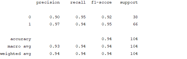
Support Vector Machine
Model Building
fromsklearn.svmimportSVC
sv=SVC(kernel='linear',random_state=0)
sv.fit(X_train,y_train

SVC(C=1.0, break_ties=False, cache_size=200, class_weight=None, coef0=0.0,
decision_function_shape='ovr', degree=3, gamma='scale', kernel='linear',
max_iter=-1, probability=False, random_state=0, shrinking=True, tol=0.001,
verbose=False)

Cross-validation using training data
fromsklearn.model_selectionimportcross_val_score
accuracies=cross_val_score(estimator=sv,X=X_train,y=y_train,cv=10)
print("accuracy is {:.2f} %".format(accuracies.mean()*100))
print("std is {:.2f} %".format(accuracies.std()*100))

Predicting the class
pre=sv.predict(X_test)

Accuracy and Confusion Matrix
svm_accuracy=accuracy_score(pre,y_test)
print("Accuracy of the model is "+str(round(accuracy_score(pre,y_test),4)*100)+str(" %"))
data={'Actual value':y_test.to_list(),'Predicted Value':pre}
df=pd.DataFrame(data)
confusion_matrix=pd.crosstab(df['Actual value'],df['Predicted Value'],rownames=['Actual'],colnames=['Predicted'])
sns.heatmap(confusion_matrix,annot=True)
plt.show()

Classification Report
fromsklearn.metricsimportclassification_report
print(classification_report(pre,y_test))

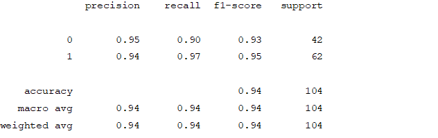
K-nearest Neighbour
Model Building
fromsklearn.neighborsimportKNeighborsClassifier
score=[]
foriinrange(1,10):

knn=KNeighborsClassifier(n_neighbors=i,metric='minkowski',p=2)
knn.fit(X_train,y_train)
pre3=knn.predict(X_test)
ans=accuracy_score(pre3,y_test)
score.append(round(100*ans,2))
print(sorted(score,reverse=True)[:5])
knnn=sorted(score,reverse=True)[:1]
[100.0, 98.08, 97.12, 97.12, 96.15]

Cross-validation using training data
fromsklearn.model_selectionimportcross_val_score
accuracies=cross_val_score(estimator=knn,X=X_train,y=y_train,cv=10)
print("accuracy is {:.2f} %".format(accuracies.mean()*100))
print("std is {:.2f} %".format(accuracies.std()*100))
accuracy is 91.11 %
std is 4.14 %

Predicting the class
pre=knn.predict(X_test)

Accuracy and Confusion Matrix
knn_accuracy=accuracy_score(pre,y_test)
print("Accuracy of the model is "+str(round(accuracy_score(pre,y_test),4)*100)+str(" %"))
data={'Actual value':y_test.to_list(),'Predicted Value':pre}
df=pd.DataFrame(data)
confusion_matrix=pd.crosstab(df['Actual value'],df['Predicted Value'],rownames=['Actual'],colnames=['Predicted'])
sns.heatmap(confusion_matrix,annot=True)
plt.show()

Classification Report
fromsklearn.metricsimportclassification_report
print(classification_report(pre,y_test))

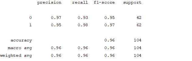
Naive Bayes
Model Building
fromsklearn.naive_bayesimportGaussianNB
gb=GaussianNB()
gb.fit(X_train,y_train)
GaussianNB(priors=None, var_smoothing=1e-09)

Cross-validation using training data
fromsklearn.model_selectionimportcross_val_score
accuracies=cross_val_score(estimator=gb,X=X_train,y=y_train,cv=10)
print("accuracy is {:.2f} %".format(accuracies.mean()*100))
print("std is {:.2f} %".format(accuracies.std()*100))
accuracy is 89.20 %
std is 3.72 %

Predicting the class
pre=gb.predict(X_test)

Accuracy and Confusion Matrix
nb_accuracy=accuracy_score(pre,y_test)
data={'Actual value':y_test.to_list(),'Predicted Value':pre}
df=pd.DataFrame(data)
confusion_matrix=pd.crosstab(df['Actual value'],df['Predicted Value'],rownames=['Actual'],colnames=['Predicted'])
sns.heatmap(confusion_matrix,annot=True)
plt.show()

Classification Report
fromsklearn.metricsimportclassification_report
print(classification_report(pre,y_test))

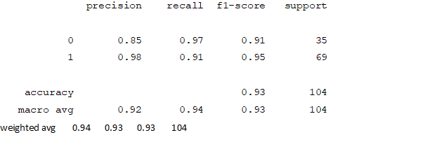
Decision Tree Classifier
Model Building
fromsklearn.treeimportDecisionTreeClassifier
dc=DecisionTreeClassifier(criterion='gini')
dc.fit(X_train,y_train)
DecisionTreeClassifier(ccp_alpha=0.0, class_weight=None, criterion='gini',
max_depth=None, max_features=None, max_leaf_nodes=None,
min_impurity_decrease=0.0, min_impurity_split=None,
min_samples_leaf=1, min_samples_split=2,
min_weight_fraction_leaf=0.0, presort='deprecated',
random_state=None, splitter='best')

Cross-validation using training data
fromsklearn.model_selectionimportcross_val_score
accuracies=cross_val_score(estimator=dc,X=X_train,y=y_train,cv=10)
print("accuracy is {:.2f} %".format(accuracies.mean()*100))
print("std is {:.2f} %".format(accuracies.std()*100))
accuracy is 95.21 %
std is 3.20 %

Predicting the class
pre=dc.predict(X_test)

Accuracy and Confusion Matrix
decision_tree=accuracy_score(pre,y_test)
data={'Actual value':y_test.to_list(),'Predicted Value':pre}
df=pd.DataFrame(data)
confusion_matrix=pd.crosstab(df['Actual value'],df['Predicted Value'],rownames=['Actual'],colnames=['Predicted'])
sns.heatmap(confusion_matrix,annot=True)
plt.show()

Classification Report
fromsklearn.metricsimportclassification_report
print(classification_report(pre,y_test))

Random Forest Classifier
Model Building
fromsklearn.ensembleimportRandomForestClassifier
estime=[]
foriinrange(1,100):
rc=RandomForestClassifier(n_estimators=i,criterion='entropy',random_state=0)
rc.fit(X_train,y_train)

Cross-valiadation using training data
fromsklearn.model_selectionimportcross_val_score
accuracies=cross_val_score(estimator=rc,X=X_train,y=y_train,cv=10)
print("accuracy is {:.2f} %".format(accuracies.mean()*100))
print("std is {:.2f} %".format(accuracies.std()*100))

accuracy is 96.90 %
std is 3.20 %

Predicting the class
pre=rc.predict(X_test)

Accuracy and Confusion Matrix
random_forest=accuracy_score(pre,y_test)
data={'Actual value':y_test.to_list(),'Predicted Value':pre}
df=pd.DataFrame(data)
confusion_matrix=pd.crosstab(df['Actual value'],df['Predicted Value'],rownames=['Actual'],colnames=['Predicted'])

sns.heatmap(confusion_matrix,annot=True)
plt.show()

Classification Report
fromsklearn.metricsimportclassification_report
print(classification_report(pre,y_test))

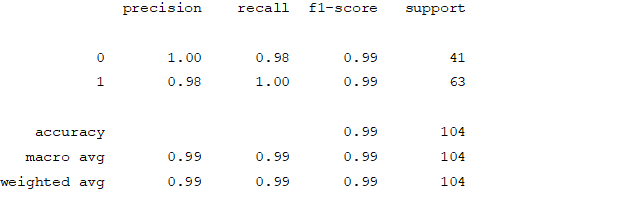
Results
print('Logistic regression:',logistic_regression)
print('svmlinear:',svm_accuracy)

print('knn:',knn_accuracy)
print('naive bayes:',nb_accuracy)
print('Decision tress:',decision_tree)
print('Random forest:',random_forest)

Logistic regression: 0.9615384615384616
svmlinear: 0.9423076923076923
knn: 0.9615384615384616
naive bayes: 0.9326923076923077
Decision tress: 0.9903846153846154
Random forest: 0.9903846153846154

9.2. Hospitalized diabetes patient’s readmission prediction – k means clustering
9.2.1. Code
Importing the relevant libraries
%matplotlibinline
importpandasaspd
importmatplotlib.pyplotasplt
importnumpyasnp
fromsklearn.clusterimportDBSCAN,KMeans
fromsklearn.manifoldimportTSNE
fromsklearn.metrics.pairwiseimportpairwise_distances
frommatplotlib.colorsimportListedColormap
importseabornassns

Reading the data
data=pd.read_csv('diabetic_data.csv')

Seeing the first 5 rows of the dataset
data.head()

Getting the number of rows and columns in the dataset
data.shape
(101766, 50)

Getting the name of the column, datatype and number of non-null values
data.info()

RangeIndex: 101766 entries, 0 to 101765
Data columns (total 50 columns):

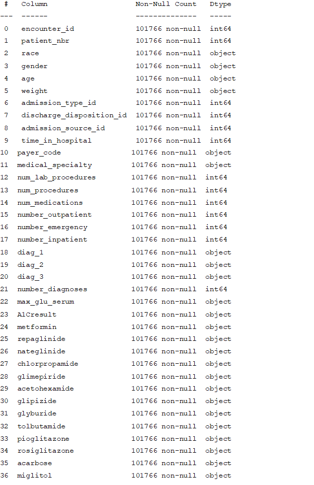
dtypes: int64(13), object(37)
memory usage: 38.8+ MB

Getting the statistical parameter values for each column
data.describe()

Analysing non-numeric columns
forcolindata.columns:
ifdata[col].dtype==object:
print(col,data[col][data[col]=='?'].count())
race 2273
gender 0
age 0
weight 98569
payer_code 40256
medical_specialty 49949
diag_1 21
diag_2 358
diag_3 1423
max_glu_serum 0
A1Cresult 0
metformin 0
repaglinide 0
nateglinide 0
chlorpropamide 0
glimepiride 0
acetohexamide 0
glipizide 0
glyburide 0
tolbutamide 0
pioglitazone 0
rosiglitazone 0
acarbose 0
miglitol 0
troglitazone 0
tolazamide 0
examide 0
citoglipton 0
insulin 0
glyburide-metformin 0
glipizide-metformin 0
glimepiride-pioglitazone 0
metformin-rosiglitazone 0
metformin-pioglitazone 0
change 0
diabetesMed 0
readmitted 0

Cleansing the date
data=data.drop(['weight','payer_code','medical_specialty'],axis=1)
drop_Idx=set(data[(data['diag_1']=='?')|(data['diag_2']=='?')|(data['diag_3']=='?')].index)
drop_Idx=drop_Idx.union(set(data[data['discharge_disposition_id']==11].index))
new_Idx=list(set(data.index)-set(drop_Idx))
data=data.iloc[new_Idx]

Getting the name of categorical features in the dataset
categorical=data.select_dtypes(include=['object'])
categorical_names=categorical.columns.values

Plotting the bar graph to get the frequency of each categories present
fig,axes=plt.subplots(nrows=7,ncols=5,figsize=(24,24))
axe=axes.ravel()
foriinrange(len(categorical_names)):
data[categorical_names[i]].value_counts().plot(ax=axe[i],kind='bar')
axe[i].set_xlabel(categorical_names[i])
axe[i].set_ylabel("frequency")
fig.tight_layout()

data=data.drop(['citoglipton','examide'],axis=1)
drop_Idx=drop_Idx.union(set(data['gender'][data['gender']=='Unknown/Invalid'].index))
new_Idx=list(set(data.index)-set(drop_Idx))

Changing categorical values into binary form
Age value is given as an interval.
Changing interval to an average value of the interval
'''
defagecategory(x):
ifx=="[0-10)”:
return5
elifx=="[10-20)":
return15
elifx=="[20-30)":
return25
elifx=="[30-40)":
return35
elifx=="[40-50)":
return45
elifx=="[50-60)":
return55
elifx=="[60-70)":
return65
elifx=="[70-80)":
return75
else:
return0
data['age']=data['age'].apply(lambdax:agecategory(x))
#Making the target variable and other variables binary
data['readmitted']=data['readmitted'].apply(lambdax:0ifx=="NO"else1)
data['change']=data['change'].apply(lambdax:0ifx=="No"else1)
data['gender']=data['gender'].apply(lambdax:0ifx=="Female"else1)
data['diabetesMed']=data['diabetesMed'].apply(lambdax:0ifx=="No"else1)
data['service_utilization']=data['number_outpatient']+data['number_emergency']+data['number_inpatient']

Analysing the number of medication changes taken by the patient
treatments=['metformin','repaglinide','nateglinide','chlorpropamide','glimepiride','acetohexamide', 'glipizide','glyburide','tolbutamide','pioglitazone','rosiglitazone','acarbose','miglitol','troglitazone',
'tolazamide','insulin','glyburide-metformin','glipizide-metformin','glimepiride-pioglitazone','metformin-rosiglitazone','metformin-pioglitazone']
$assigning a value of 0 if there are not undergoing treatment and assigning 1 even if they are taking \
#increasing/decreasing/steady dosage
foriintreatments:
data[i]=data[i].apply(lambdax:0ifx=="No"else1)
#finding out total number of treatments taken by patient
data['treatments_taken']=np.zeros((len(data['metformin'])))
forcolintreatments:
data['treatments_taken']+=data[col]

Number of medication changed
Converting data into binary form
data['A1Cresult']=data['A1Cresult'].apply(lambdax:0ifx=="None"else(1ifx=="Norm"else2))
data['max_glu_serum']=data['max_glu_serum'].apply(lambdax:0ifx=="None"else(1ifx=="Norm"else2))

Categorising the diagnosis into 9 classes
defgetCategor(x):
if'V'instr(x)or'E'instr(x):
return0
x=float(x)
if(x>=390andx<=459)ornp.floor(x)==785:
return1
elif(x>=460andx<=519)ornp.floor(x)==786:
return2
elif(x>=520andx<=579)ornp.floor(x)==787:
return3
elifnp.floor(x)==250:
return4
elifx>=800andx<=999:
return5
elifx>=710andx<=739:
return6
elif(x>=580andx<=629)ornp.floor(x)==788:
return7
elifx>=140andx<=239:
return8
else:
return0
#changing the values into categories
data['diag_1_category']=data['diag_1'].apply(lambdax:getCategor(x))

Check for readmitted patients and remove all visits other than the 1st visit
patients=data['patient_nbr']
data[patients.isin(patients[patients.duplicated()])]

#dropping the patients encounters other than 1st visit
data=data.drop_duplicates(subset=['patient_nbr'],keep='first')
data.shape
(69343, 48)
data['admission_type_id']=data['admission_type_id'].astype('object')
data['admission_source_id']=data['admission_source_id'].astype('object')
data['discharge_disposition_id']=data['discharge_disposition_id'].astype('object')
data['diag_1_category']=data['diag_1_category'].astype('object')
data['max_glu_serum']=data['max_glu_serum'].astype('object')
data['A1Cresult']=data['A1Cresult'].astype('object')

Removing the unnecessary columns from the data
delete_columns = ['encounter_id','patient_nbr','number_outpatient','number_emergency','number_inpatient', 'metformin','repaglinide','nateglinide','chlorpropamide','glimepiride','acetohexamide','glipizide', 'glyburide','tolbutamide','pioglitazone','rosiglitazone','acarbose','miglitol','troglitazone', 'tolazamide','insulin','glyburide-metformin','glipizide-metformin','glimepiride-pioglitazone',' metformin-rosiglitazone','metformin-pioglitazone','diag_1']
data.drop(delete_columns, inplace=True, axis=1)
#creating a list of categorical and numeric lists
categorical=data.select_dtypes(include=['object'])
numeric=data.select_dtypes(exclude=['object'])
print(categorical.columns.values)
print(numeric.columns.values)
['race' 'admission_type_id' 'discharge_disposition_id'
'admission_source_id' 'diag_2' 'diag_3' 'max_glu_serum' 'A1Cresult'
'diag_1_category']
['gender' 'age' 'time_in_hospital' 'num_lab_procedures' 'num_procedures'
'num_medications' 'number_diagnoses' 'change' 'diabetesMed' 'readmitted'
'service_utilization' 'treatments_taken']
# creating dummies for all the categorical variables and deleting the original columns
nominal_columns = ['race', 'admission_type_id', 'discharge_disposition_id','admission_source_id' ,'diag_1_category'\
, 'max_glu_serum', 'A1Cresult']
dummy_df = pd.get_dummies(data[nominal_columns])
data = pd.concat([data, dummy_df], axis=1)
data = data.drop(nominal_columns, axis=1)

Clustering Algorithm
processed_data=pd.read_csv('processed_data.csv')
KMClusterers={}# what an inelegant word
KMClusterers['Parent']=KMeans(n_clusters=2,random_state=0,max_iter=300)
Clusters={}
Clusters['KM parent']=pd.Series(KMClusterers['Parent'].fit_predict(processed_data),
index=processed_data.index,name='KM parent')
sns.lmplot(x='PC_0',y='PC_1',col='KM parent',data=processed_data.join(Clusters['KM parent']),palette='colorblind',
hue='KM parent',fit_reg=False,height=5,aspect=1.4);
plt.title('Projection of dataset onto first two principal components');

processed_data_km_subset = processed_data.loc[Clusters['KM parent']==0, :]
KMClusterers['Child']=KMeans(n_clusters=2,random_state=0,max_iter=300)
Clusters['KM child']=pd.Series(KMClusterers['Child'].fit_predict(processed_data_km_subset),
index=processed_data_km_subset.index,name='KM child');
Clusters['KM']=Clusters['KM child']+2
Clusters['KM']=pd.concat([Clusters['KM'],
Clusters['KM parent'].loc[Clusters['KM parent'].index.drop(Clusters['KM child'].index)]],
axis=0)
Clusters['KM'].name='KM clusters'
sns.lmplot(x='PC_0',y='PC_2',data=processed_data.join(Clusters['KM']),
palette='colorblind',hue='KM clusters',fit_reg=False,height=5,aspect=2.5);
plt.title('Projection of dataset onto the first two principal components');

Dataset=pd.read_csv('Dataset_trimmed.csv')
# Make datasets consisting of samples from each cluster
Dataset_km1=Dataset.loc[Clusters['KM']==1,:]
Dataset_km2=Dataset.loc[Clusters['KM']==2,:]
Dataset_km3=Dataset.loc[Clusters['KM']==3,:]
# Create a dataframe containing the means of each feature for each of the above datasets
k1_mus=Dataset_km1.describe().loc['mean',:]
k2_mus=Dataset_km2.describe().loc['mean',:]
k3_mus=Dataset_km3.describe().loc['mean',:]
kn_mus=pd.concat([k1_mus,k2_mus,k3_mus],axis=1)
kn_mus.columns=['Cluster 1','Cluster 2','Cluster 3']
kn_mus=kn_mus.apply(func=(lambdarow:row/(row.mean())),axis=1)
cblind=[sns.color_palette('colorblind')[0],sns.color_palette('colorblind')[1],sns.color_palette('colorblind')[2]]
kn_mus.plot.bar(cmap=ListedColormap(cblind),figsize=(15,7),title='Cluster feature means');

kn_mus.apply(func=(lambdarow:row/(row.mean())),axis=1)# Scaling the means to better represent cluster differences

defnormalised_value_counts(series):
returnseries.value_counts()/len(series)
f,ax=plt.subplots(1,3,sharex=False,sharey=False,figsize=(16,6))
N_bars=np.arange(len(Dataset_km1.diag_1.unique()))*2
normalised_value_counts(Dataset_km1.diag_1).plot(kind='barh',ax=ax[0],
color=sns.color_palette('colorblind')[0])
ax[0].set_title('Cluster '+str(0+1))
N_bars=np.arange(len(Dataset_km2.diag_2.unique()))*2
normalised_value_counts(Dataset_km1.diag_2).plot(kind='barh',ax=ax[1],
color=sns.color_palette('colorblind')[1])
ax[1].set_title('Cluster '+str(1+1))
N_bars=np.arange(len(Dataset_km3.diag_3.unique()))*2
normalised_value_counts(Dataset_km3.diag_3).plot(kind='barh',ax=ax[2],
color=sns.color_palette('colorblind')[2])
ax[2].set_title('Cluster '+str(2+1))
plt.tight_layout()