data analysis assignment on data mining and modelling for real world use

Question

Task: How to use data analysis assignment research methods to review, analyse and report data results

Answer

Question 1
Descriptive statistics
Variable 1: Advertisement type?
Variable 2: Number of clicks?

The difference between sample used on this data analysis assignment meansx ?_1 -x ?_2 = 253.2037 – 190.9565 = 62.25
This implies that the difference in mean number of clicks between emotional and informational advertisement type is 62.25 units. Relevant graph to represent the predicted shape of histogram

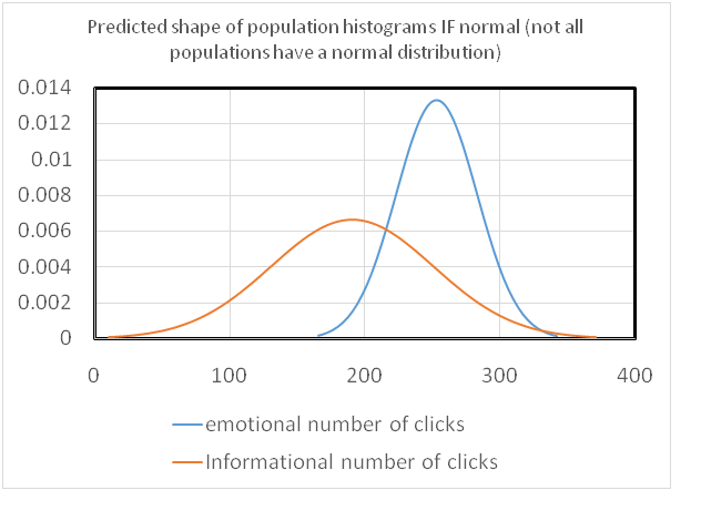
Comparison identified on this data analysis assignment: It is evident from the peaks of the histogram that the mean number of clicks is maximum for emotional advertisement type as compare with the informational advertisement type. Further, the spread is greater for informational in comparison with emotional advertisement type. The shape of histogram of informational advertisement type does not show normal distribution because of the high spread as comparison with population’s distribution. Large sample size needs to be taken into account to represent the true underlying population. However, as per the shape and spread of histogram of emotional advertisement type, it can be said that it follows normal distribution.

Question 2
Descriptive statistics
Variable 1: Independent variable: Number of clicks?”
Variable 2: Dependent variable: Number of purchase?”

Scatter plot

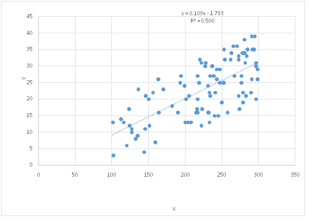
The correlation coefficient r = 0.7075

The positive value of r generated on this data analysis assignment is clear indication of the positive relationship between number of clicks and number of purchase. Further, the extend of the magnitude is nearby 0.75 which shows that the net strength of the relationship between them is moderate to strong. As the number of clicks increases then their corresponding number of purchase will also be increased.

Regression line to predict the number of purchase
Y = a + b X
Y = -1.7936 + 0.1097X
“Number of purchase?” = -1.7936 +( 0.1097 * “Number of clicks?”)

Number of clicks is given as 2000 now number of purchase
“Number of purchase?” = -1.7936 +( 0.1097 *2000) = 217.59 or 218
For 2000 number of clicks increases the corresponding number of purchase will be 218.

Question 3
Descriptive statistics (data set 2)

Variable 1: “Reality, pregnant or not pregnant”
Variable 2: “Test result, positive or negative”

The difference between sample proportions p ?_1 -p ?_2= 83.11% or -83.11%
The significant difference between the sample proportion indicates that the pregnancy test is considered to be significantly effective in the diagnosis process.

Descriptive statistics (data set 3)
Variable 1: “Reality, pregnant or not pregnant”
Variable 2: “Test result, positive or negative”

The difference between sample proportions p ?_1 -p ?_2 = 91.62% or -91.62%

It is evident from the above two relationship estimation that the difference between the sample proportion for larger sample (data set 3) comes out to be higher as compared with the small sample (data set 2). Hence, the conclusion can be drawn that the data set 3 results more accurate result than data set 2. Thus, data set 3 is better.

Question 4
Assessing the accuracy of sample estimate of PILOT study

Sample proportion (pregnant, test positive) p= 0.9474

Standard error of the sample proportion = ?((p(1-p)/n)) = ? ((0.9474(1-0.9474)/100)) = 0.0223

Assessing the accuracy of sample estimate of LARGER study

Sample proportion (pregnant, test positive) p= 0.9779

Standard error of the sample proportion = ?((p(1-p)/n)) = ? ((0.9779(1-0.9779)/1000)) = 0.00465

Question 5
Relevant output from Question 1of data analysis assignment

For informational appeal type of advertisement, 95% confidence interval for number of clicks
Degree of freedom = n-1 = 54-1 = 53
The t value = 2.006

Lower Limit = x – (t*s/n0.5) = 253.2037 – 2.006*29.94/540.5 = 245.03
Upper Limit = x + (t*s/n0.5)= 253.2037 + 2.006*29.94/540.5 = 261.374
Based on this, the 95% confidence interval for population mean number of clicks for information type advertisement is 245.03< µ < 261.37.

For emotional appeal type of advertisement, 95% confidence interval for number of clicks
Degree of freedom = n-1 = 46 -1 = 45
The t value = 2.014
Lower Limit = x – t*s/n0.5 = 190.9565 – 2.016*60/460.5 = 173.13
Upper Limit = x + t*s/n0.5 = 190.9565 – 2.016*60/460.5 = 208.77

Based on this, the 95% confidence interval for population mean number of clicks for emotional type advertisement is 173.13< µ< 208.77.

Question 6
Computer output from excel to determine the evidence to support the claim regarding the presence of relationship between advertisement type” and “number of clicks” is shown below.

Based on the above output, the 95% confidence interval for the difference between population mean number of clicks of informational and emotional type advertisement is 42.779 < µd< 208.77.

The p value for the hypothesis test = 0.00
Significance level = 5% (Assuming)
Observation: The p value (two tailed) of the hypothesis test is lower than 5%
Result: Reject null hypothesis (H0) and accept alternative hypothesis (H1)
Therefore, the strong relationship possessed between variables. Hence, significant difference between exists in mean number of clicks between informational and emotional type advertisement.

Question 7
Computer output from excel to determine the evidence to support the claim regarding the existence of relationship between “Number of clicks”and“Number of purchase” is shown below.

Based on the above output, the 95% confidence interval for the slope coefficient between variables number of clicks and number of purchase is 0.0877< ?< 0.1317.

The p value for the hypothesis test = 0.00
Significance level = 5% (Assuming)

Observation: The p value (two tailed) of the hypothesis test is lower than 5% Result: Reject null hypothesis (H0) and accept alternative hypothesis (H1) Therefore, the slope coefficient is termed as significant and a statistically significant positive relationship exists between number of clicks and number of purchase.

Question 8
Computer output from excel to determine the evidence of the claim regarding the existence of relationship between “test result positive or negative?” and “reality pregnant or not pregnant?” is shown below.

Based on the above output, the 95% confidence interval for the difference of population proportion is 0.6364 <(p1-p2)<1.0258.

The p value for the hypothesis test of this data analysis assignment= 0.00
Significance level = 5% (Assuming)

Observation: The p value (two sided) of the hypothesis test is lower than 5% Result: Reject null hypothesis (H0) and accept alternative hypothesis (H1) There is strong evidence to conclude the difference in the population proportion and association between “test result positive or negative?” and “reality pregnant or not pregnant?

Question 9
For the given task, the video selected is “Introduction to Linear Regression” (Link:https://www.youtube.com/watch?v=TU2t1HDwVuA) The objective of the video is to allow a broad level understanding of linear regression. It has been defined as the linear relationship whereby one or more independent variables may be used to predict the value of a dependent variable. A general relationship is obtained which then can be used to determine the dependent variable value based on different values of the independent variable. In a process called as interpolation, the independent variable values are within the range of the values used while determining regression model and the corresponding values of dependent variable are determined using the regression model. However, in extrapolation the independent variable values outside the range are considered. Since the linear relationship may not apply to such values, hence there is a greater likelihood of error in such forecasts. 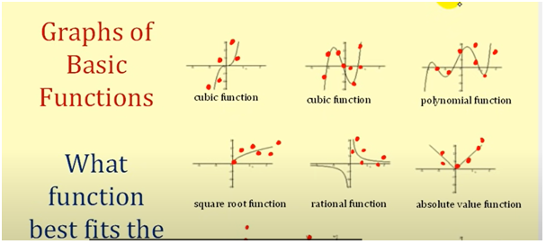The linear regression process used on this data analysis assignmentstarts with the scatter plot which plots the independent and dependent variable on the X and Y axis. The objective of this plot is to see the broad pattern in the points so as to determine whether a linear relationship is indeed present between the variables or not. It is necessary that the relationship is necessarily linear and the non-linear patterns may arise which would indicate towards the following functions.

If the pattern based on the scatter plot is found to be broadly linear, then it makes sense to find the correlation coefficient. This coefficient highlights the strength and nature of the relationship between the underlying variables. The magnitude of the correlation coefficient ( 0 to 1) is indicative of the linear relationship strength with 0 being the weakest and 1 being the strongest. A positive correlation coefficient would hint that both the variables tend to move in the same direction while a negative correlation coefficient would hint at the variables moving in the opposite direction.

Another useful parameter is the coefficient of determination or R2. It can be computed using the correlation coefficient since it is the square of the correlation coefficient. The coefficient of determination highlights whether the underlying model is a good fit or not for the given data. This is because it is a measure of the predictive ability of the regression model. If the regression model used on this data analysis assignmenthas low predictive ability, then usually it would indicate poor fit since the resultant residuals would be high.