
Artificial Intelligence Assignment: Predictive Power & Accuracy of Machine Learning Methods
Question
Task
Write a detailed report on artificial intelligence assignment critically discussing about the predictive power and accuracy of different machine learning methods.
Answer
Introduction:
As per the research on artificial intelligence assignment, it is stated that companies have become data driven and Artificial Intelligence has become the foundation for it. Machine learning a sub-branch of artificial intelligence, used the sample data to build a mathematical model and it will be named as training data, for a precise and accurate prediction and validate the results using a validation model. Moreover, Machine learning is related to computational statistics, which focuses on making predictions using computers. Due to wide variety application of machine learning in analytics, business and forecasting area and machine learning is also referred to as predictive analytics.
In this study we focus on the predictive power and accuracy of different machine learning methods. The focuses will be on the Logistic regression, Navies Bayes Classification and K Near Neighbour techniques .Our aim is to study the predictive power and accuracy of the above three techniques. For that, the data have been taken from the second edition of the Computational intelligence and Learning (CoIL) competition Challenge in the Year 2000, organized by CoIL cluster, and four EU funded Networks of Excellence has been cooperated with it. Their major focuses will be on the areas of evolutionary computing (EvoNet) , neural networks (NeuroNet), fuzzy systems (ERUDIT), and machine learning (MLNet). This dateset which is based on real world business problem of Car insurance policy has been developedand contributed by Peter van der Putten of the Dutch data mining company Sentient Machine Research, Baarsjesweg 224 1058 AA Amsterdam The Netherlands +31 20 6186927 putten@liacs.nl and. TIC (The Insurance Company) Benchmark Homepage (http://www.liacs.nl/~putten/library/cc2000) was donated on March 7, 2000. The detailed report of the data can be assessing from the P. van der Putten and M. van Someren (eds). CoIL Challenge 2000: The Insurance Company Case published by Sentient Machine Research, Amsterdam. Also a Leiden Institute of Advanced Computer Science Technical Report 2000-09. June 22, 2000.
Method:
In this study, the dataset has been taken from the real customer response of d 86 predictors that measures the demographic characteristics for over 5866 individuals from Computational intelligence and Learning (CoIL) competition Challenge in the Year 2000. The data is directly taken from the insurance company to predict and assess whether an individual is interested in the caravan insurance policy. To increase the market of an insurance policy, it is very crucial to study the response variance is 'purchase' that indicates whether or not a given individual purchases a car insurance policy. From the dataset it was found that out of 5866, only 348 individuals have purchased the policy. Fig 1: depict the summary of customers with and without Caravan insurance policy.
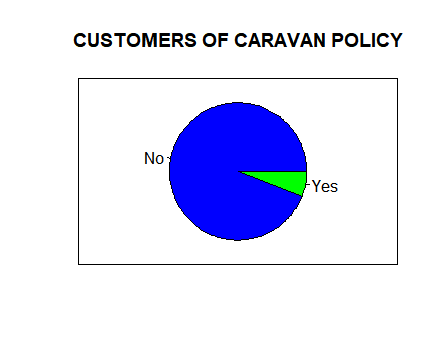
Fig 1: Customers of Caravan policy
As a pre-processing step, check for the missing values, outliers and multicollinearity were done. There was no evidence of missing data and outliers and multicollinearity. A bivariate analysis has been used to check whether the relationship between the customers who purchased caravan policy with their sociodemographic variables and variables indicating the existences of other polices. From chi square analysis it was found that there is an association that
- There was significant association between the customer who has taken police with the demographic variables like the age, type of family they belongs to, family income and power type.
- The customers with boat policies has not purchased the caravan policy [chisquared = 620.71, df = 2, p-value < 2.2e-16].
- The customers with boat policies has not purchased the social security policy [chi square = 286.94, df = 1, p-value < 2.2e-16].
- Those who have purchased Caravan policy has been paying car policy of premium average from $ 1000, $ 4999. [Chisquared = 218.84, df = 2, p-value < 2.2e-16].
- Those who have purchased Caravan policy has taken one fire policy [chi squared = 218.84, df = 2, p-value < 2.2e-16].
For the purpose of prediction, the data has been partitioned into training test that contains 5000 description about the customers and a test set which consist of 4000 customers. The prediction task is to know the response of a given individual for purchasing the car insurance policy.
Findings:
a. Logistic Regression
A Logistic regression was used as a prediction model to determine the factors that affect the purchase of purchases a car insurance policy. Since the outcome variable is a categorical variable with two possible outcomes Yes and No, a Binomial logistic regression was performed. The results of the logistic regression are presented below;
Call:
glm(formula = Purchase ~ MOSHOOFD + MSKB1 + PWAPART, family = binomial(link = "logit"), data = tr)
Deviance Residuals:
Min 1Q Median 3Q Max
-0.7591 -0.3796 -0.3222 -0.2449 2.7517
Coefficients:
Estimate Std. Error z value Pr(>|z|)
(Intercept) -2.61150 0.21697 -12.036 < 2e-16 ***
MOSHOOFD -0.12578 0.02826 -4.451 8.57e-06 ***
MSKB1 0.10615 0.05499 1.930 0.0536 .
PWAPART 0.34260 0.08070 4.245 2.18e-05 ***
Signif. codes: 0 ‘***’ 0.001 ‘**’ 0.01 ‘*’ 0.05 ‘.’ 0.1 ‘ ’ 1
(Dispersion parameter for binomial family taken to be 1)
Null deviance: 1301.2 on 2910 degrees of freedom
Residual deviance: 1254.6 on 2907 degrees of freedom
AIC: 1262.6
Number of Fisher Scoring iterations: 6
From, the above result the model is has a good fit with Residual deviance: 1254.6 on 2907 degrees of freedom and AIC: 1262.6.
Multicollinearity of the model was checked using the Variance Inflamation factor. If the value of Variance Inflamation factor (VIF), is greater than 10, the presence of multicollinearity has been detected. For the above model, the VIF value is less than 5 and can conclude that there is no presence of multicollinearity.
vif(lgmodel)
MOSHOOFD MSKB1 PWAPART
1.029716 1.029719 1.000016
Now the validation of above model is predicted by creating the training set and 'test' or the 'validation' set. The model prediction is done by using the training data and the validation test is used to validate the model performance. For the validation purpose the dataset has been portioned using the common split ratio is 70:30. The above model contains a good fit and the same model is used for the prediction of train set. And the summary statistic for the validation model is given below;
summary (lg_predictions)
Min. 1st Qu. Median Mean 3rd Qu. Max.
0.02045 0.03213 0.05302 0.05885 0.07208 0.25036
The accuracy of the validated model was determined by Receiver operating curve. The Area Under the Curve (AUC), will give whether the model has the discrimination property or not. For the validation model, the Area Under the Curve (AUC) is 0.606. This indicates that the validation model has the discriminate power of 60 percentages when compared with the training dataset. The Receiver operating curve has been plotted below;
auc
[1] 0.6057173
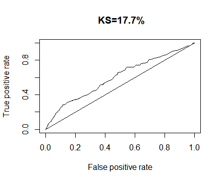
Gini Index is used to measures how much better is the validation model is performing compared to training model. For Gini coefficient, a value of 0% indicates a model which is no better than random or in other words no prediction power. And a Gini value of 100% will indicate a perfect model- it will accurately predict good and Bad 100%. For the model, the Gini Value is 0.288, which indicated a 28 % predictive power of the validation model when compared with random model.
gini
[1] 0.2888877
b. Naive Bayes classifiers
Naive Bayes classifier is based on Bayes’ Theorem and consists of a collection of classification algorithms. It is a family of algorithms in which all the algorithm share a common principle in which each pair of features that has been classified will be independent of each other. Most of assumptions that have been used to make the Naive Bayes algorithm are not generally correct and often works well in practice in real-world situations. After the application of Naïve Bayes classifier, the results are as follows;
Naive Bayes Classifier for Discrete Predictors
Call:
naiveBayes.default(x = X, y = Y, laplace = laplace)
A-priori probabilities:
Y
No Yes
0.9412573 0.0587427
Conditional probabilities:
MOSHOOFD
Y [,1] [,2]
No 5.824818 2.835126
Yes 4.690058 3.056885
MSKB1
Y [,1] [,2]
No 1.593796 1.339557
Yes 1.906433 1.511725
PWAPART
Y [,1] [,2]
No 0.7474453 0.9510149
Yes 1.0818713 1.0025080
## Naive Bayes Confusion Matrix
>confusionMatrix(nb_predictions,te$Purchase)
Confusion Matrix and Statistics
Reference
Prediction No Yes
No 2738 173
Yes 0 0
Accuracy : 0.9406
95% CI : (0.9314, 0.9489)
No Information Rate : 0.9406
P-Value [Acc > NIR] : 0.5202
Kappa : 0
Mcnemar's Test P-Value : <2e-16
Sensitivity : 1.0000
Specificity : 0.0000
Pos Pred Value : 0.9406
Neg Pred Value : NaN
Prevalence : 0.9406
Detection Rate : 0.9406
Detection Prevalence : 1.0000
Balanced Accuracy : 0.5000
'Positive' Class : No
The accuracy of Naive Bayes Classifier is about 94 %. Ie Accuracy : 0.9406 [95% CI : (0.9314, 0.9489)]. The Sensitivity of the model is 100 percentage and specificity is 0 %.
c. K Nearest Neighbouhood (KNN):
K Nearest Neighbors (KNN) is a non-parametric test that can be considered as the one of the most important classification algorithms in the field of Machine Learning. It can be used as a supervision model that can be used for classification as well as a regression model with intense application in data mining, pattern recognition, and intrusion detection.
The results of K Nearest Neighbouhood (KNN) are presented below;
knnmod
k-Nearest Neighbors
2911 samples
3 predictor
2 classes: 'No', 'Yes'
Pre-processing: centered (3), scaled (3)
Resampling: Cross-Validated (10 fold)
Summary of sample sizes: 2621, 2620, 2620, 2620, 2619, 2621, ...
Resampling results across tuning parameters:
k Accuracy Kappa
2 0.9388584 -0.001901387
3 0.9398858 0.000000000
4 0.9398858 0.000000000
5 0.9398858 0.000000000
6 0.9398858 0.000000000
7 0.9398858 0.000000000
8 0.9398858 0.000000000
9 0.9398858 0.000000000
10 0.9398858 0.000000000
11 0.9398858 0.000000000
12 0.9398858 0.000000000
13 0.9398858 0.000000000
14 0.9398858 0.000000000
15 0.9398858 0.000000000
16 0.9398858 0.000000000
17 0.9398858 0.000000000
18 0.9398858 0.000000000
19 0.9398858 0.000000000
20 0.9398858 0.000000000
Accuracy was used to select the optimal model using the largest value.
The final value used for the model was k = 20.
>knn_predictions <- predict(knnmod,te)
># KNN Confusion Matrix
>confusionMatrix(knn_predictions,te$Purchase)
Confusion Matrix and Statistics
Reference
Prediction No Yes
No 2738 173
Yes 0 0
Accuracy : 0.9406
95% CI : (0.9314, 0.9489)
No Information Rate : 0.9406
P-Value [Acc > NIR] : 0.5202
Kappa : 0
Mcnemar's Test P-Value : <2e-16
Sensitivity : 1.0000
Specificity : 0.0000
Pos Pred Value : 0.9406
Neg Pred Value : NaN
Prevalence : 0.9406
Detection Rate : 0.9406
Detection Prevalence : 1.0000
Balanced Accuracy : 0.5000
'Positive' Class : No
The accuracy of K Nearest Neighbour (KNN)is about 94.1 %. Ie Accuracy : 0.9406 [95% CI : (0.9314, 0.9489)]. The Sensitivity of the model is 100 percentages and specificity is 0 %.
Among the three models Naive Bayes Classifier and K Nearest Neighbour (KNN) have the same level of accuracy with 94%. But in real life scenario K Nearest Neighbour (KNN) would be more suitable.
Model Tuning
Tuning is the process of maximizing a model’s performance without over fitting and by using “hyperparameters” it has been accomplished in the machine learning. Bagging and boosting are the techniques used for model tuning. Bagging refers to the way in which the variance is decreased by creating another data set and boosting refers to the adjustment of data using some weight. The weight is taken from the last observation of the classifier.
In this scenario, we have used the bagging technique to reduce the variance and see the accuracy.
The results are as follows;
Bagging classification trees with 25 bootstrap replications
Call: bagging.data.frame(formula = Purchase ~ MOSHOOFD + MSKB1 + PWAPART,
data = tr, control = rpart.control(maxdepth = 5, minsplit = 4))
> #Prediction
> bag.pred <- predict(mod.bagging, te)
> ## Bagging Confusion Matrix
> confusionMatrix(bag.pred,te$Purchase)
Confusion Matrix and Statistics
Reference
Prediction No Yes
No 2734 177
Yes 0 0
Accuracy : 0.9392
95% CI : (0.9299, 0.9476)
No Information Rate : 0.9392
P-Value [Acc > NIR] : 0.52
Kappa : 0
Mcnemar's Test P-Value : <2e-16
Sensitivity : 1.0000
Specificity : 0.0000
Pos Pred Value : 0.9392
Neg Pred Value : NaN
Prevalence : 0.9392
Detection Rate : 0.9392
Detection Prevalence : 1.0000
Balanced Accuracy : 0.5000
'Positive' Class : No
By the bagging method, the accuracy of model has reduced to 93.9 %.
Conclusion:
Among the prediction methods discussed above within this artificial intelligence assignment, K Nearest Neighbour method, has predicted the validation model with an accuracy of 94%. KNN method will be considered as one of the most appropriate method as it the nonparametric test that does not assumes any Gaussian distribution.
Appendix: R code
## importing dataset
install.packages("ISLR")
library (ISLR)
summary(Caravan)
#check missing values
sum(is.na(Caravan))
## No of policy holders
noofpolicy <-table(Caravan$Purchase)
noofpolicy
## pie chart for the policy holders
colors=c("blue","green")
col=colors
pie(noofpolicy,main = "CUSTOMERS OF CARAVAN POLICY",col=colors)
box()
## outlier check
hist(Caravan$MOSTYPE)
hist(Caravan$MGEMLEEF)
hist(Caravan$MOSHOOFD)
hist(Caravan$MRELGE)
# bivaraite analyis - DEMOGRAPHICS
customertype <-table(Caravan$MOSTYPE[Caravan$Purchase=="Yes"])
customertype;
chisq.test(customertype)
age <-table(Caravan$MGEMLEEF[Caravan$Purchase=="Yes"])
age <-table(Caravan$MGEMLEEF[Caravan$Purchase=="Yes"])
chisq.test(age)
income<-table(Caravan$MINKGEM[Caravan$Purchase=="Yes"])
chisq.test(income)
# bivaraite analyis - Chi-square
a <-table(Caravan$APLEZIER[Caravan$Purchase=="Yes"])
a;
chisq.test(a)
b<-table(Caravan$ABYSTAND[Caravan$Purchase=="Yes"])
b;
chisq.test(b)
c<-table(Caravan$ABRAND[Caravan$Purchase=="Yes"])
c;
chisq.test(c)
d<-table(Caravan$ABRAND[Caravan$Purchase=="Yes"])
d;
chisq.test(d)
# Data partition
set.seed(101)
library(caret)
library(DMwR)
Carnavas.ori<- Caravan
set.seed(99)
tr <- Carnavas.ori[sample(row.names(Carnavas.ori), size = round(nrow(Carnavas.ori)*0.5)),]
te <- Carnavas.ori[!(row.names(Carnavas.ori) %in% row.names(tr)), ]
tr1 <- tr
te1 <- te
te2 <-te
#PREDICTION USING Logistic regression
library(ggplot2)
library(MASS)
library(splines)
library(mgcv)
library(crossval)
set.seed(1)
lgmodel <- glm(formula= Purchase ~ MOSHOOFD + MSKB1+PWAPART, data = tr,
family = binomial(link = "logit"))
summary(lgmodel)
summary(lgmodel$fitted.values)
# Variation Inflation Factor (Multicollinearity)
vif(lgmodel)
### Prediction for test data using the final model
lg_predictions <- predict(lgmodel,te,type="response")
lg_predictions
summary (lg_predictions $ fitted.values)
## Logistic Confusion Matrix
y_pred_numl <- ifelse(lg_predictions = 2)
y_predl <- factor(y_pred_numl, levels=c(0, 1))
confusionMatrix(y_predl,te$Purchase)
############Model Performance Measures for Logistic
Regression####################
library(ROCR)
pred.lg <- prediction(lg_predictions, te$Purchase)
perf.lg <- performance(pred.lg, "tpr", "fpr")
summary (perf.lg)
perf.lg
plot(perf.lg)
KS <- max(attr(perf.lg, 'y.values')[[1]]-attr(perf.lg, 'x.values')[[1]])
KS
plot(perf.lg,main=paste0(' KS=',round(KS*100,1),'%'))
lines(x = c(0,1),y=c(0,1))
## Area Under Curve
auc <- performance(pred.lg,"auc");
auc <- as.numeric(auc@y.values)
auc
## Gini Coefficient
library(ineq)
gini = ineq(lg_predictions, type="Gini")
gini
library(e1071)
set.seed(1)
nbmodel <- naiveBayes(Purchase ~ MOSHOOFD + MSKB1+PWAPART , data=tr)
nbmodel
nb_predictions <- predict(nbmodel,te)
## Naive Bayes Confusion Matrix
confusionMatrix(nb_predictions,te$Purchase)
#KNN
library(class)
trControl <- trainControl(method = "cv", number = 10)
knnmod <- caret::train(Purchase ~ MOSHOOFD + MSKB1+PWAPART ,
method = "knn",
tuneGrid = expand.grid(k = 2:20),
trControl = trControl,
metric = "Accuracy",
preProcess = c("center","scale"),
data = tr)
knnmod
knn_predictions <- predict(knnmod,te)
# KNN Confusion Matrix
confusionMatrix(knn_predictions,te$Purchase)
# Bagging
library(gbm)
library(xgboost)
library(caret)
library(ipred)
library(plyr)
library(rpart)
mod.bagging <- bagging(Purchase ~ MOSHOOFD + MSKB1+PWAPART ,
data=tr,
control=rpart.control(maxdepth=5, minsplit=4))
mod.bagging
#Prediction
bag.pred <- predict(mod.bagging, te)
bag.pred
## Bagging Confusion Matrix
confusionMatrix(bag.pred,te$Purchase)
# Boosting
tr$Purchase <- as.character(tr$Purchase)
mod.boost <- gbm(Purchase ~ .,data=tr, distribution=
"bernoulli",n.trees =5000 , interaction.depth =4, shrinkage=0.01)
summary(mod.boost)
#Prediction
boost.pred <- predict(mod.boost, test,n.trees =5000, type="response")
## Boosting Confusion Matrix
y_pred_num <- ifelse(boost.pred > 0.5, 1, 0)
y_pred <- factor(y_pred_num, levels=c(0, 1))
table(y_pred,te$Purchase)
confusionMatrix(y_pred,te$Purchase)