(PUN105) Statistics assignment analysing the country-level COVID-19 data using statistical methods

Question

Task: Your task is to write the statistical methods and results sections of a statistics assignmentthat focuses on analysis of country-level COVID-19 data. You are required to include both descriptive and inferential statistics. Provide your analysis and interpretation of the results generated.

Answer

Statistical methodology for the statistics assignment Dataset Description
Numerical Approach
Table 1 of the statistics assignmentshows all the variables in the dataset and its datatype.

Table 1. Variables and their data types
From table 1, it is clear that there are a total nine variables in the dataset. Out of nine, seven are floats, and the other two are categorical and string.

Graphical Approach for the statistics assignment
Histogram is the graphical representation of the distribution of the data. Figure 1 and 2 in the statistics assignmentshows the histogram plot for people vaccinated per 100 and new cases per million respectively.

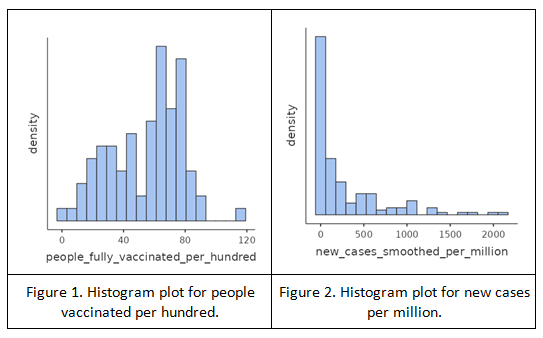
From figure 1. It is clear that the distribution of people fully vaccinated per hundred is binodal while distribution of new cases per million is unimodal with right skewed. Similarly, the distribution of regions is almost an uniform distribution. The distribution of gdp per capita is unimodal and right skewed, for life expectancy it is unimodal and left skewed. The distribution for stringency index is unimodal, new deaths per million is unimodal and right skewed.

Central Tendency mentioned in the statistics assignment

Mean
It is the arithmetic average of the measurement in a dataset. It gets influenced by an outlier very easily.

Median
It is the central value, 50% of the dataset lies above that value and 50% of the dataset lies below it. It is influenced by the outlier.

Mode
It is the most frequent or probable value in the dataset.

By looking at the mean and median value, we can say whether there are outliers in the dataset. Mean and median value should be very close to each other. If this is the case then there are outliers in the dataset. In Covid-19 dataset, the mean and median age is 32 and 32.1 respectively. So we can conclude in the statistics assignmentthat there is no outlier present. Similarly for gdp per capita, the mean and median value is 21538 and 15246. There is a very large difference in these values. Thus we can conclude that there are outliers for this variable. By same reasoning, region, life expectancy, human development index, people fully vaccinated, stringency index does not have any outliers. New cases per million and new deaths per million have outliers.

Skewness and kurtosis
If the skewness value is greater than +1.0 then the distribution is right skewed. If the skewness value is less than -1.0 then the distribution is left skewed.

For kurtosis, if the value is greater than + 1.0, the distribution is leptokurtic. If the value is less than -1.0, the distribution is platykurtic.
Thus gdp per capita, new cases per million, new deaths per million are right skewed since its value is greater than +1.0.
Region and median age distribution is platykurtic since its value is less than -1.0. GDP per capita, new cases per million, new deaths per million have distribution leptokurtic since they have kurtosis values more +1.0.

Results of the statistics assignment
To compare the DCR of high and low GDP countries, we grouped the data based on the GDP for this statistics assignment. Then we calculated the mean DCR for the country with low GDP and DCR for the country with high GDP. The mean DCR for low GDP countries is 28.35 and DR for high GDP countries is 13.15. Thus we can conclude from the statistics assignmentthat the mean DCR of high GDP countries is less than the DCR of low GDP countries. The mean of DCR for all the countries is 21.27. Thus, we can say that there is a significant difference in the DCR for low GDP countries and DCR of high GDP countries.

There are four regions in our dataset for the statistics assignment. These regions are Europe, Africa, America and Asia Pacific. We have compared the stringency index of these four regions. The figure 3 shows the bar plot of the mean stringency index for the four regions.

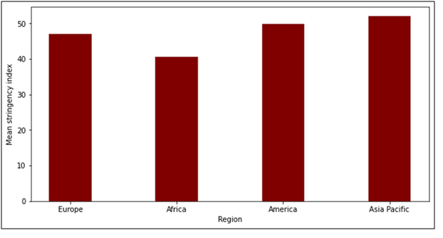
Figure 3. Stringency index of different regions

From the plot in the statistics assignment, we can see that there is not much difference between the mean stringency values. There is no significant difference in the stringency values. The maximum mean stringency index is for Asia Pacific and minimum stringency value is for Africa.

Next we investigated whether there is any relationship between the vaccinated group and the regions. Vaccinated group is a derived variable which is obtained from people fully vaccinated per hundred. If the value of people fully vaccinated per 100 is less than 40 then we call it a low vaccinated region. If the value of people fully vaccinated is more than 40, we call it a highly vaccinated region. Figure 4 in the statistics assignmentshows the bar plot for the vaccinated group based on the regions.

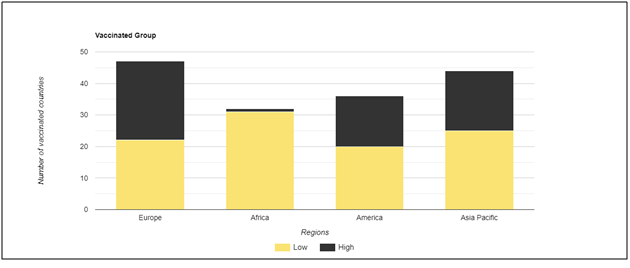
Figure 4. Vaccinated group based on regions

The vaccinated group can be either high or low based on people fully vaccinated per hundred. To find the relationship between the vaccinated group and regions, we grouped all the regions based on the vaccination level. From the plot mentioned in thev, we can see that Europe has 25 countries which are highly vaccinated and 22 countries that are low vaccinated. Thus Europe has 53.16% of countries highly vaccinated while 46.24% countries are low vaccinated. For Africa we can see that there is only one country that is highly vaccinated while 31 countries are low vaccinated. Thus in Africa, 3% of the countries are highly vaccinated while 97% of the countries are low vaccinated. For America, we can see that 16 countries are highly vaccinated while 20 countries are low vaccinated. Thus we can say that 44% of the countries are highly vaccinated and 54% of the countries are low vaccinated. For the Asia Pacific region, we can see that there are 19 countries that are highly vaccinated and 25 countries that are low vaccinated. Thus we can say that there are 43% countries that are highly vaccinated and 57% of the countries are low vaccinated countries. By comparing we can say that Europe has the most highly vaccinated countries while Africa has the least. Thus we can say from the statistics assignmentthat there is a significant relationship between the regions and the vaccinated group.

To build the multivariable model for predicting the dependent variable DCR using independent variables like region, median age etc, we use linear regression. We used GDP level, median age, life expectancy and stringency index to build the multivariable model. We compare the results of these models using r-squared scores. For the first model, we used GDP level as an independent variable and DCR as the dependent variable. The r-squared value obtained for this model is 0.1158. For the second model, we used life expectancy as an independent variable and DCR as a dependent variable. The r-squared value obtained for this model is 0.1384. For the third model, we used median age in the statistics assignmentas an independent variable and DCR as a dependent variable. The r-squared value obtained for this model is 0.074. For the fourth model, we used stringency index as an independent variable and DCR as a dependent variable. The r-squared value for this model is 0.0005. Figure 5 shows the r-squared value for all the four models.

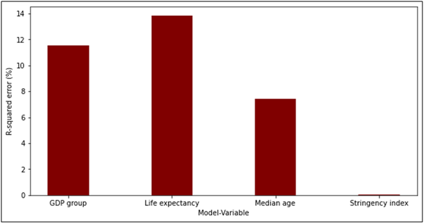
Figure 5. R-squared values

From figure 5 in the statistics assignment, we can say that life expectancy has the best r-squared value followed by the GDP group. Stringency index has the worst R-squared error. Interpretation of R-squared value for life expectancy is done such that there are 14% chances of the changeability of the dependent output attribute can be explained by the model while the remaining 86% of the variability is still unaccounted for. Similarly the interpretation of R-squared value for stringency index is done such that there is 0.05% chances of the changeability of the dependent output attribute can be explained by the model while the remaining 99.45% of the variability is still unaccounted for. Similarly the interpretation of R-squared value for GDP group is done such that there is 11.56% chances of the changeability of the dependent output attribute can be explained by the model while the remaining 88.44% of the variability is still unaccounted for. Similarly the interpretation of R-squared value for median age is done such that there are 7.40% chances of the changeability of the dependent output attribute can be explained by the model while the remaining 92.60% of the variability is still unaccounted for. Next we investigated whether the GDP group is an effect modifier of the relationship between DCR and life expectancy. To investigate this in the statistics assignment, we build a model with only one independent variable that is life expectancy and another model in which we use two independent variables that are life expectancy and GDP group. Figure 6 shows the R-squared value with only life expectancy and life expectancy along with GDP.

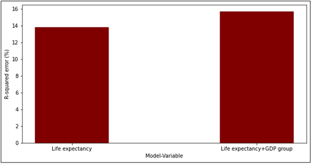
Figure 6. R-squared value

From the figure 6 we can see that the R-squared value of the life expectancy model alone is 13.47% whereas the R-squared value of the model with life expectancy and GDP group is 15.71%. The interpretation of the R-squared value for life expectancy model is that there are 13.47% chances of the changeability of the dependent output attribute can be explained by the model while the remaining 86.53% of the variability is still unaccounted for. The interpretation of the R-squared value for life expectancy and GDP group model is that there are 15.77% chances of the changeability of the dependent output attribute can be explained in the statistics assignmentby the model while the remaining 84.23% of the variability is still unaccounted for.
To build the minimal model, we used five variables that gave the best r-squared value. These variables are region, GDP per capita, life expectancy, new cases per million, and new deaths per million. The R-squared value of the minimal model is 0.2231. The interpretation of the R-squared value for the minimal model is that there are 22.31% chances of the changeability of the dependent output attribute can be explained by the model while the remaining 87.69% of the variability is still unaccounted for. The equation for the minimal model is given below.

minimal model = 2.75*region-0.0039*gdp per capita-0.79*life expectancy- 0.07*new cases per million+1.87*new death per million

From the equation in the statistics assignmentwe can see that the region and new death per million coefficient value is the highest. They will have the maximum impact on the equation. While the gdp per capita and new cases per million has the minimum coefficient value thus having the least impact on the equation.

If we build the maximal model wherein we use all the variables then the R-squared value will be 0.2338. The interpretation of the R-squared value for the maxial model is that there are 23.38% chances of the changeability of the dependent output attribute can be explained by the model while the remaining 76.62% of the variability is still unaccounted for. The figure 7 in the statistics assignmentshows the bar plot for the r-squared value of the minimal and the maximal model.

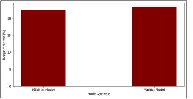
Figure 7. R-squared value for minimal and maximal model

From figure 7 in the statistics assignment, we can see that there is not much difference between the r-squared value of the minimal and the maximal model.