Statistics Assignment Tutorial Statistics for Business Decisions

Question

Task

The questions to be answered in this statistics assignment are;

Week 2 Question 1:

In your own words, differentiate the following statistical terminologies with some examples.

a. Population Parameter and Sample Statistic

b. Descriptive Statistics and Inferential Statistics

c. Nominal Scale and Ordinal Scale

d. Primary Data Source and Secondary Data Source

Week 3 Question 1:

Data showing the population by state in millions of people follow (The World Almanac, 2012).

a. Develop a frequency distribution, a percent frequency distribution, and a histogram. Use a class width of 2.5 million.

b. Does there appear to be any skewness in the distribution? Explain.

c. What observations can you make about the population of the 50 states?

Week 4 Question 2:
Forty-three percent of Americans use social media and other websites to voice their opinions about television programs (the Huffington Post, November 23, 2011). Below are the results of a survey of 1364 individuals who were asked if they use social media and other websites to voice their opinions about Television programs

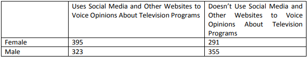
a. Show a joint probability table.

b. What is the probability a respondent is female?

c. What is the conditional probability a respondent uses social media and other websites to voice opinions about television programs given the respondent is female?

d. Let F denote the event that the respondent is female and A denote the event that the respondent uses social media and other websites to voice opinions about television programs. Are events F and A independent?

Week 5 Question 3:
The average starting salary for this year's graduates at a large university (LU) is $20,000 with a standard deviation of $8,000. Furthermore, it is known that the starting salaries are normally distributed.

• What is the probability that a randomly selected LU graduate will have a starting salary of at least $30,400?
• What is the probability that a randomly selected LU graduate will have a salary of exactly $30,400?
• Individuals with starting salaries of less than $15600 receive a low income tax break. What percentage of the graduates will receive the tax break?
• If 189 of the recent graduates have salaries of at least $32240, how many students graduated this year from this university?

Week 6 Question 3:
The College Board reported the following mean scores for the three parts of the SAT (The World Almanac, 2009):

Critical reading 502

Mathematics 515

Writing 494

Assume that the population standard deviation on each part of the test is 100.

a) What is the probability that a random sample of 90 test takers will provide a sample mean test score within 10 points of the population mean of 502 on the Critical reading part of the test?

b) What is the probability that a random sample of 90 test takers will provide a sample mean test score within 10 points of the population mean of 515 on the Mathematics part of the test? Compare this probability to the value computed in part (a).

Answer

Week 2 Answer 1
a. As per the investigation on statistics assignment, population parameter characterizes a population (Teja, and Reddy, 2018, p. 416-418). All the measures of central tendency (mean, median, mode etc.) and measures of dispersion (range, inter-quartile range, standard deviation etc.) when measured using all the observations from the population are called population parameters. However, it is quite a monumental task to calculate descriptive measures using all observations of a large population until the population is small enough to be practically explored and assessed completely.

For example, calculation of average level of blood pressure level of all Australian citizens is a herculean task. Nevertheless, evaluation similar statistical measure for all college students (considering all college students as the population) seems a viable option. Generally, population parameters are known from previous facts or are guessed by the researcher.

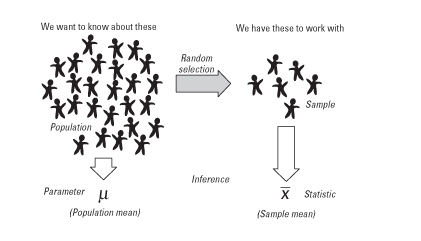
Figure 1: Illustration of Population Parameter and Sample Statistic

Sample statistic is always easier to calculated using all the observations from the particular sample. Sample statistic exemplifies the sample features and helps us draw inferences about the population. An underlined condition is that the sample should be drawn randomly from the population so that properties of the population remains preserved in the sample.

For, example, average blood sugar level and its standard deviation of all the patients in a hospital are sample statistics. In case of skewed distribution, median and inter-quartile range can also be evaluated.

b. Descriptive statistics can be categorized as measures of central tendency and measures of dispersion (Amrhein, Trafimow, and Greenland, 2019, p. 262-270). Also, graphical analysis alongside tabular presentation of data is also considered as descriptive statistics since data can be easily interpreted through these measures. Although, descriptive statistics provide clear summary and understanding of the sample or population data, it cannot help in inferring any conclusive and confirmative decisions about the population.

For instance, a two-way table can help us in understand the relation between two categorical variables, Also, a histogram or a boxplot alongside the average and standard deviation with a standard deviation of measures can immensely help in understanding the pattern of the sample data. Average mark of students in mathematics as 78 with standard deviation of 8 provides a rough idea that 95% of the students have scored between 62 and 94. However, it is not possible to conclude whether average mark of students was significantly different from 82.

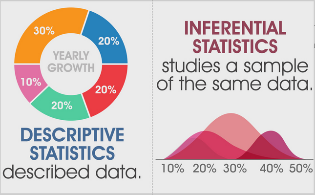
Figure 2: Descriptive statistics and inferential statistics explanation

Inferential statistics is a branch of confirmatory and conclusive statistics that assists a researcher to draw conclusion about the population from sample descriptions, compare two populations, and even draw conclusions on hypothetical assumptions about the population. ANOVA, Chi-Square, T-test, Regression, Kruskal-Wallis test, Mann Witney U test are some statistical tests which are used for drawing decisions.

For instance, average marks in mathematics of students from a particular section of class ten as 78 with standard deviation of 8 can be tested against hypothetical claim that average marks of all students in mathematics is 82 using one-sample t-test with 95% level of confidence (probability).

c. Nominal, Ordinal, Interval, and Ratio are four scales of measurement of a data. Nominal and Ordinal can measure categorical data, whereas Interval and Ration scale measure continuous quantitative data (Doszy?, 2017, p. 75-84). Nominal scale measures those categorical variables where the categories are not related by any specific order. Colour of flowers, gender, and ethnicity are few variables which are measured by nominal scale.

For example, choice of caffeinated drinks with categories as Tea, Coffee, and Red bull is a nominal scale variable where the categories cannot be numerical compared using any kind of ordering.

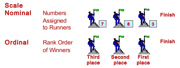
Figure 3: Comparison between Nominal and Ordinal scales

Ordinal scale variable measures those categorical variables which have sense of ordering, if not meaningful numerical values. Categories of ordinal measurement can be compared among themselves and ranked according to their order. Opinion on government policies, attitude of family members towards a cooked dish, age groups are few instances of ordinal measurements.

Example: Temperature measured in cold, hot, and very hot categories is example of an ordinal variable. Here, numerical value of a category has no practical meaning, but ranking of cold as 1, hot as 2, and very hot as 3 indicates a comparative ordering.

d. Primary data sources are those origins of data that generate original and first hand data. Interviews, survey, field observations, and experiments are sources of primary data. Data collection becomes a costly and time consuming job (Merson et al., 2018, p.e965). Chances of missing and invalid responses are also present in the primary data which has to be cleaned for any research purpose. Reliability and validity of primary data sources is also a concern among many in the field of data collection. This first hand data sources are generally used to solve a problem at hand.

Collection of student feedbacks about a teacher in a university is primary data collection, where students are the primary data source. Record of coverage of footpaths in locality is a primary data collection where the field survey measurement is the primary data source.

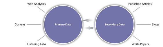
Figure 4: Sources of Primary and Secondary Research Data

Published articles, government and organizational websites, blogs, social media platforms, white papers, books are few sources of secondary data. In order to research on a project not at hand we tend to collect secondary data. Generally, these types of data are kept cleaned for the purpose of future research works or study. Some advantages in collecting data from the secondary sources are less time consumption, almost negligible costs, and high reliability.

Study of advancement of space research can be easily made through success and failure assessment of space missions. For this purpose, data can be collected from secondary data sources such as newspapers, magazines or website of space agencies (NASA, ISRO etc.).

Week 3: Answer 1
a. Frequency Distribution:

Table 1: Frequency distribution of population (million)

Percentage Frequency Distribution:

Table 2: Percentage Frequency distribution of population (million)

Percentage Histogram:

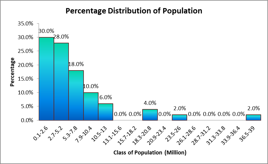
Figure 5: Histogram of Percentage Frequency distribution of population (million)

b. There appears to be high positive / right skewness in the data. The distribution is far from normal shaped curve, and few high outlier observations have created as long tail of the distribution. Figure5 reveals that 8% (four states) states have population highly greater than other states. Therefore, the distribution has a right tail and a right skewness.

c. Distribution of population is evident from the frequency distribution tables and the histogram. It is noted that 30% of the states have population between 0.1 million and 2.6 million. Other 28% states have populace between 2.7 million and 5.2 million. Hence, more than half of the 50 states (58%) have population less than 5.2 million. Among the rest 44% states, 18% have population between 5.3 million and 7.8 million, and 10% have population in-between 7.9 million and 10.4 million. Again, 6% states (3 states) with populace more than 10.5 million were some of the most populated states in the list. But, 8% (four states) states have population abnormally higher (outliers) compared to the other states causing a right skewed distribution of population.

Week 4 Answer 2

Table 3: Two-way table for gender and use of social media for opinion

Table 4: Joint probability calculation details (correct to 2 decimal places)

a. The joint probability table from Table2 can be presented as below:

Table 5: Joint probability (correct to 2 decimal places)

b. Probability of a respondent being female is 0.5 (From Table3). Calculation is in Table2: (395/1364 = 0.29) + (291/1364 = 0.21) = (696/1364 = 0.50)

c. Conditional probability: Prob.(Respondent uses social media to voice opinion about TV / female) = Prob.(Respondent uses social media to voice opinion about TV and a female) / Prob.(Respondent is a female) = 0.29 / 0.5 = 0.58

Required conditional probability = 0.58

d. F = Respondent is a female: A = Respondent uses social media to voice opinion about TV

Condition of independence: Prob. (Respondent uses social media to voice opinion on TV and a female) = Prob. (Respondent is a female) * Prob. (Respondent uses social media to voice opinion about TV)

From Table3:

Prob. (Respondent uses social media to voice opinion on TV and a female) = 0.29

Prob. (Respondent is a female) * Prob. (Respondent uses social media to voice opinion about TV) = 0.5 * 0.53 = 0.26

Hence, Prob. (Respondent uses social media to voice opinion on TV and a female) ?Prob. (Respondent is a female) * Prob. (Respondent uses social media to voice opinion about TV)

So, A and F are not independent.

Week 5: Answer 3
Random Variable: X = Starting salary for this year's LU graduates

Mean = µ = $20,000: Standard Deviation = ? = $8,000

Standard Normal Variable Z = (X - µ) / ?

a. Prob. (X >= $30,400) = 1 - Prob. (X< $30,400) =1 – Prob. (Z< (30,400 – 20,000) / 8000) ) = 1 – Prob. (Z< 1.3) = 1 – 0.90320 = 0.0968 (Ross, p. 131- 140) Required probability = 0.097

b. Prob. (X = $30,400) = 0 (probability of an exact value of X for a continuous distribution is considered to be zero).

c. Prob. (X < $15,600) =Prob. (Z< (15,600 – 20,000) / 8000)) = Prob. (Z < -0.55) = 0.29116 (using standard normal table).

Hence, almost 29.12% students will get tax break.

d. Let there be N number of students. So, N * Prob. (X >= $32,240) = 189

Now, Prob. (X >= $32,240) =1 - Prob. (X< $32,240) =1 – Prob. (Z< (32,240 – 20,000) / 8000)) = 1 – Prob. (Z< 1.53) = 1 – 0.93699 = 0.06301.

Hence, N * 0.06301 = 189 => N = 3000

Total 3000 students graduated this year from LU University.

Week 6: Answer 3
X1: Critical reading: µ1 = 502, ?1 = 100, n1 = 90

X2: Mathematics: µ2 = 515, ?2 = 100, n2 = 90

X3: Writing: µ3 = 494, ?3 = 100

Standard Normal Variable Z = (X - µ) /(? /?n)

a. Prob. (|(X - µ1)|< 10) = Prob. (|Z| < 10/ (100/?90)) = Prob. (|Z|< 0.949) = 2 * Prob. (|Z|< 0.95) = 2* (0.82894 – 0.5) = 0.65788

Required probability = 0.66

b. Prob. (|(X - µ2)|< 10) = Prob. (|Z| < 10/ (100/?90)) = Prob. (|Z|< 0.949) = 2 * Prob. (|Z|< 0.95) = 2* (0.82894 – 0.5) = 0.65788

Required probability = 0.66

Similarity: Both probabilities are same since in both cases deviation from mean, standard deviation, and sample sizes are same. Hence, probabilities of achieving score within 10 points of average marks of mathematics and critical reading are same for 90 test takers.

References
Amrhein, V., Trafimow, D. and Greenland, S., 2019. Inferential statistics as descriptive statistics: There is no replication crisis if we don’t expect replication. The American Statistician, 73(sup1), pp.262-270.

Doszy?, M., 2017. Statistical determination of impact of property attributes for weak measurement scales. Real Estate Management and Valuation, 25(4), pp.75-84.

Merson, L., Guérin, P.J., Barnes, K.I., Ntoumi, F. and Gaye, O., 2018. Secondary analysis and participation of those at the data source. Statistics assignment The Lancet Global Health, 6(9), p.e965.

Ross, A., 2017. Area Under the Normal Curve. In Pedagogy and Content in Middle and High School Mathematics (pp. 131-140). Brill Sense.

Teja, S.G.S. and Reddy, H.P., 2018. Inferential Statistics for Data Science. International Journal for Research in Applied Science & Engineering Technology (IJRASET), 6(7), pp.416-418.