Statistics Assignment Interpreting Statistical Scenarios

Question

Task

The questions to be answered in this statistics assignment are;

Week 7 Question 2
A local health centre noted that in a sample of 400 patients, 80 were referred to them by the local hospital.

a. Provide a 95% confidence interval for all the patients who are referred to the health centre by the hospital.

b. What sample size would be required to estimate the proportion of all hospital referrals to the health centre with a margin of error of 0.04 or less at 95% confidence?

Week 8 Question 1
The average starting salary of students who graduated from colleges of Business in 2009 was $48,400. A sample of 100 graduates of 2010 showed an average starting salary of $50,000. Assume the standard deviation of the population is known to be $8000. We want to determine whether or not there has been a significant increase in the starting salaries.

Step 1. Statement of the hypothesis

Step 2. Standardised test statistic formula

Step 3. State the level of significance

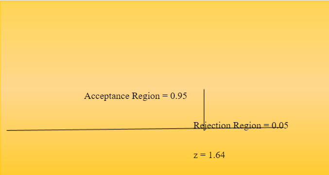
Step 4. Decision Rule (Draw a bell to show rejection zone)

Step 5. Calculation of the statistic

Step 6. Conclusion

Week 9 Question 3
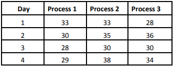
The data in the table below presents the hourly quantity of production for three lines of production processes over the first 4 days in XYZ Company. Answer the questions based on the Excel Output given below.

a. State the null and alternative hypothesis for single factor ANOVA.

b. State the decision rule (? = 0.05).

c. Calculate the test statistic.

d. Make a decision.

Week 10 Question 2
Personal wealth tends to increase with age as older individuals have had more opportunities to earn and invest than younger individuals. The following data were obtained from a random sample of eight individuals and records their total wealth (Y) and their current age (X).

A part of the output of a regression analysis of Y against X using Excel is given below:

a. State the estimated regression line and interpret the slope coefficient.

b. What is the estimated total personal wealth when a person is 50 years old?

c. What is the value of the coefficient of determination? Interpret it.

d. Test whether there is a significant relationship between wealth and age at the 10% significance level. Perform the test using the following six steps.

Step 1. Statement of the hypotheses

Step 2. Standardised test statistic

Step 3. Level of significance

Step 4. Decision Rule

Step 5. Calculation of test statistic

Step 6. Conclusion

Week 11 Question 3
A student used multiple regression analysis to study how family spending (y) is influenced by income (x1), family size (x2), and additionsto savings(x3). The variables y, x1, and x3 are measured in thousands of dollars. The following results were obtained.

a. Write out the estimated regression equation for the relationship between the variables.

b. Compute coefficient of determination. What can you say about the strength of this relationship?

c. Carry out a test to determine whether y is significantly related to the independent variables. Use a 5% level of significance.

d. Carry out a test to see if x3 and y are significantly related. Use a 5% level of significance.

Answer

Week 7: Statistics Assignment Question 2
N = 400 (total sample space), x = 80 (referred locals)

Hence, observed p = 80/ 400 = 0.2 (ratio of referred locals)

a. Confidence Interval = 95% =>z-score = 1.96

Standard Error (SE) = p1-pN=0.21-0.2400 = 0.02

Margin of error (ME) = 1.96 * 0.02 = 0.0392

Confidence Interval = [0.2 – 0.0392, 0.2 + 0.0392] = [0.1608, 0.2392](Sedgwick, 2015, p.h1113)

95% CI for referred patients to health centre is between [0.16, 0.24], or between 16% and 24% (approximately).

b. Required Margin of error (ME) = 0.04, Confidence Interval = 95% => z-score = 1.96

Now, ME = SE / ?N, where N is sample size.

Standard Error (SE) = p1-pN=0.21-0.2N

Hence, ME = Z20.21-0.2N=> 0.04 = 1.96*0.21-0.2N

=>?N = 1.960.04*0.2*0.8=19.6

=> N = 19.6 * 19.6 = 384.16 ? 385(Suresh, and Chandrashekara, 2012, p.7)

Therefore, minimum 385 sample size would be required to achieve a margin of error of 0.04 at 95% confidence interval.

Week 8: Question 1
Given Information:

Variable = X = Average Starting Salary

Population in 2009: Mean = µ = $48,400, Standard Deviation = ? = $8000

Sample in 2010: Mean = _ x = $50,000, Size = n = 100

Step 1:
Null hypothesis: H0: (µ2009 = µ2010):Average starting salary of graduates in 2009 and 2010 were same.

Alternate hypothesis: There was a significant increase in average starting salary of graduates in 2010 from average starting salary in 2009 (right tailed test).

Step 2:
Choice of test was Z-test for known population mean and standard deviation.

The test statistics: Z=_ X-? n

Step 3:
Level of Significance = 5% =>? = 0.05

Step 4:
The null hypothesis will be rejected if z-calculated > z-critical at 5% level.

Step 5:
Test Statistic =Z=_ X-? n = 50,000-48,0008000100=2000800= 2.5

Hence, z-calculated = 2.5 > z-critical = 1.64 at 5% level.

Step 6:
As the calculated statistic value is greater than the critical value of the statistic, the null hypothesis is rejected at 5% level(Pandis, 2015, pp.350-351). Hence, average starting salary of graduates have significantly increased in 2010 from 2009.

Week 9: Question 3
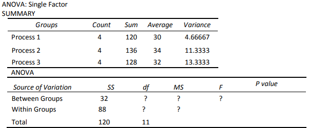
One-waysingle factor ANOVA(Quirk, 2012, pp. 163-179)

a. Null hypothesis: H0: (µ1 = µ2 = µ3):Average hourly production quantities for three production processes were same.

Alternate hypothesis: There is at least one production process that has significantly different average hourly production quantity compared to that of other processes.

b. Decision Rule: At 5% level of significant, the null hypothesis will be rejected if calculated F-statistic from the ANOVA table is greater than critical F (2, 9) statistic where 2 and 9 were numerator and denominator degrees of freedom.

c. Test Statistic:
Between groups: df = k – 1 = 3 – 1 = 2

Within groups = df = 12 – 3 = 9

Between groups: MSB = SSB / (k – 1) = 32 / 2 = 16

Within groups = MSE = SSE/ (n – k) = 88 / 9 = 9.78

F-statistic = MSB/ MSE = 16/ 9.78 = 1.64

d. The calculated F (2, 9) = 1.64 < critical F (2, 9) = 4.256

e. Hence, null hypothesis failed to get rejected at % level. Therefore, it can be concluded that average hourly production quantities for three production processes were statistically same.

Week 10: Question 2
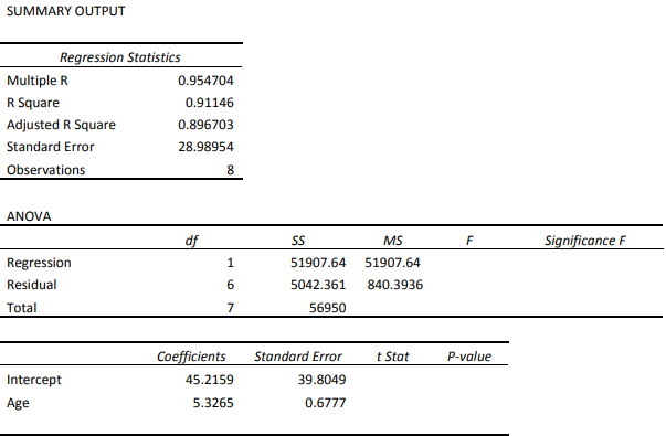
Regression: Total wealth (‘000s of dollars) on Age (Years)

a. Estimated Regression Line: Y (Total Wealth) = 45.22 + 5.33 * Age (Years)

Slope coefficient = 5.33 (correct to two decimal places)

Interpretation: It was estimated that increase in age by one year of an individual increases his/ her total wealth by approximately 5.33 thousand dollars.

b. Age = 50 years

Estimated Regression Line: Y (Total Wealth) = 45.22 + 5.33 * Age (Years)

Estimate Total Wealth = 45.22 + 5.33 * 50 = 311.72

Therefore, estimated total wealth of a 50 year old individual would be approximately 312 thousand dollars.

c. Coefficient of determination = R2 = 0.91

Interpretation: Age of an individual was able to explain or predict almost 91% variation of total wealth of that person. Hence, 91% of total wealth of an individual was successfully predicted by age of that person.

d. Hypothesis Testing: Relation between age and wealth (Nau, 2014)
Step 1:

Null hypothesis: H0: (? = 0):There was no relation between age and wealth of an individual.

Alternate hypothesis: H0: (?? 0): There was statistically significant relation between age and wealth of an individual.

Step 2:
Test Statistic: t-stat = Coefficient / Standard Error

Step 3:
Level of significance = 5% =>? = 0.05

Step 4:
Decision Rule:

If calculated t-statistic > t-critical at n – 2 = 8 – 2 = 6 degrees of freedom, null hypothesis is rejected at 5% level.

Step 5:
Test Statistic: t-stat = 5.3265/ 0.6777 = 7.859

Critical t-statistic at 5% level = 2.44

Step 6:
Conclusion: As the calculated t-statistic = 7.86 > critical t-statistic = 2.44 at 6 degrees of freedom, the null hypothesis is rejected at 5% level. Therefore, there was statistically significant relation between age and wealth of an individual.

Week 11: Question 3
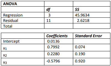
Multiple Regression Analysis:

a. Regression equation:

Y (Family spending) = 0.014 + 0.799 * X1 (Income) + 0.228 * X2 (Family Size) – 0.580 * X3 (Addition to Savings)

b. Computation of coefficient of determination:
From ANOVA table: SSE = 2.6218, SST = 45.9634

R2 = 1 – SSE/ SST = 1 – 2.6218/ 45.9634 = 0.943 (3 decimal places)

Coefficient of correlation = R = ?0.943 = 0.971

Hence, the linear relation between the variables was very strong (almost perfect).

Hence, income, family size, and addition to savings were able to explain or predict 94.3% variation of family spending.

c. Hypothesis Testing: Correlation of Y with X1, X2, and X3(Burks, Randolph, and Seida, 2019, pp.61-79)

Null hypothesis: H0: (?1 = ?2 = ?3 = 0):Family spending has no correlation with Income, Family Size, and Addition to Savings.

Alternate hypothesis: HA: (At least one ?j? 0): Family spending has significant correlation with at least one of the independent variables Income, Family Size, and Addition to Savings.

Level of significance: 5%=>? = 0.05

Choice of Test: F-test

Decision Rule: If calculated F-value > critical F-value then the null hypothesis is rejected at 5% level.

Test statistics:

Calculated F-value = MSTMSE=45.96342.6218=17.53

Critical F-value = F (3 , 11) = 3.587

Decision: As calculated F-value > critical F-value, the null hypothesis is rejected at 5% level. Hence, Family spending has significant correlation with at least one of the independent variables Income, Family Size, and Addition to Savings.

d. Hypothesis Testing: Correlation of Y with X3

Null hypothesis: H0: (?3 = 0): Family spending has no correlation with Addition to Savings.

Alternate hypothesis: HA: (?3? 0): Family spending has significant correlation with Addition to Savings.

Level of significance: 5%=>? = 0.05

Choice of Test: T-test
Decision Rule: If calculated t-value < critical t-value then the null hypothesis is rejected at 5% level.

Test statistics:
Calculated t-value = -0.5796 / 0.920 = -0.63

Critical t-value at df = 11 = - 2.2

Decision: As calculated t-value > critical t-value, the null hypothesis failed to get rejected at 5% level. Hence, Family spending has no significant correlation with Addition to Savings.

References
Burks, J.J., Randolph, D.W. and Seida, J.A., 2019. Modeling and interpreting regressions with interactions. Journal of Accounting Literature, 42, pp.61-79.

Nau, R., 2014. Notes on linear regression analysis. Fuqua School of Business, Duke University website. http://people. duke. edu/~ rnau/Notes_on_linear_regression_analysis--Robert_Nau. pdf (accessed June 14, 2020).

Pandis, N., 2015. Comparison of 2 means (independent z test or independent t test). Statistics assignment American journal of orthodontics and dentofacial orthopedics, 148(2), pp.350-351.

Quirk, T.J., 2012. One-way analysis of variance (ANOVA). In Excel 2007 for Educational and Psychological Statistics (pp. 163-179). Springer, New York, NY.

Sedgwick, P., 2015. Confidence intervals, P values, and statistical significance. Bmj, 350, p.h1113.

Suresh, K.P. and Chandrashekara, S., 2012. Sample size estimation and power analysis for clinical research studies. Journal of human reproductive sciences, 5(1), p.7.